Logistic regression is a classification method that predicts observed binary variables \(Y \in \{0, 1\}\) from explanatory variables X.
\(Y \sim \mathcal{B}\): Y follows a Bernoulli distribution.
It is a member of the Generalized linear models: logistic regression applies a sigmoid function on linearly regressed inputs.
The logistic regression does not require assumptions as strong as the linear regression. However to obtain good estimations some assumptions must be respected:
1) Independence of observations: \(\mathrm{Cov}(\varepsilon_i, \varepsilon_j) = 0 \; (i \neq j)\)
2) Linear relation between explanatory variables and the logit of the observed variables must be linear. Let \(p=P(Y=1 \vert X)\), thus we want \(\log\frac{p}{1-p}\) to have a linear relation to X,
3) No collinearity: explanatory variables are linearly independent ie the matrix X is of maximal rank - \(rank = n_{parameters}\),
4) No strongly influential outlier
1) Plot of residuals
2) Box-Tidwell Test
3) VIF
4) Cook distance + standardized residuals
This part has been written based on this toward data science post
First let’s introduce the sigmoid function:
\[g(z)=\frac{1}{1+e^{-z}}\]The sigmoid function insures that the output of the logistic regression model are between 0 and 1 ie they represent a probability. See the page for Sigmoid function for more details.
Using the sigmoid function, let’s define \(h_\beta(X)\) as \(g(\beta X)\):
\[h_\beta(X)=g(\beta X)=\frac{1}{1+e^{-\beta X}}\]The Logit function is the inverse of the sigmoid function:
\[logit(p) = \log\left(\frac{p}{1-p}\right) \;\;\; \forall p \in ]0, 1[\]See the page for Logit function for more details.
Logistic regression is from the family of regression models as the relation between the input data \(X\) and the logit of the predictions made by the model is linear. In other terms, the logit of the prediction of the model \(\beta X\) are a linear combination of the variables \(X\).
This is immediate using the formula of the logistic regression and of the logit function:
\[logit(h_\beta(X)) = logit(g(\beta X)) = \beta X\]As \(logit(g(x)) = x\).
Logit means logistic units and is also called log-odds.
To understand what log-odds is it is important to important what odds is.
Odds is simply the ratio between the probability of success over the probability of failure:
\[odds(p) = \frac{p}{1-p} = \exp(logit(p))\]Where:
Note that this value is positive but can be greater than 1.
For example when throwing a dice, the probability to get a 4 is \(1/6\) however the odds of getting a 4 is \(\frac{1/6}{5/6}=\frac{1}{5}\). It is simply the probability of winning (to get a 4) over the probability of losing (to get another number).
Let’s define the probability of Y given X in a logistic regression:
\[\begin{cases} P(Y=1 \vert X; \beta)=h_\beta(X)\\ P(Y=0 \vert X; \beta)=1-h_\beta(X)\\ \end{cases}\]The probability for \(Y=1\) is \(h_\beta(X)\) and for \(Y=0\) it is \(1-h_\beta(X)\).
Hence the above definition can be summarize in one line using the property of the power function:
\[P(Y \vert X; \beta)=\left(h_\beta(X)\right)^Y\left(1-h_\beta(X)\right)^{1-Y}\]If \(Y=1\) the right part is equal to 1 and thus we obtain \(h_\beta(X)\) and if \(Y=0\) the left part is equal to 1 and thus we obtain \(1-h_\beta(X)\).
Maximum likelihood is used to calibrate the parameter \(\beta\) and Gradient Descent is used to make the optimization. Let’s define the likelihood function \(L(\beta)\) as follow:
\[\begin{eqnarray} L(\beta) &&= P(Y \vert X; \beta) \\ &&= \prod_{j=1}^{n_{pop}}P(Y^{(j)} \vert X^{(j)}; \beta) \\ &&= \prod_{j=1}^{n_{pop}}\left(h_\beta(X^{(j)})\right)^{Y^{(j)}}\left(1 - h_\beta(X^{(j)})\right)^{1-Y^{(j)}} \\ \end{eqnarray}\]It can also be wrote:
\[\begin{eqnarray} L(\beta) &&= \prod_{j:Y^{(j)}=1} h_\beta(X^{(j)}) \; \prod_{j:Y^{(j)}=0} \left(1 - h_\beta(X^{(j)})\right) \\ &&= \prod_{j=1}^{n_{pop}}\left(h_\beta(X^{(j)})\right)^{Y^{(j)}}\left(1 - h_\beta(X^{(j)})\right)^{1-Y^{(j)}} \end{eqnarray}\]Now let’s define the log likelihood function:
\[\begin{eqnarray} l(\beta) &&= \log L(\beta) \\ &&= \log \left[\prod_{j=1}^{n_{pop}}P(Y^{(j)} \vert X^{(j)}; \beta)\right] \\ &&= \sum_{j=1}^{n_{pop}}Y^{(j)} \log h_\beta(X^{(j)})+(1-Y^{(j)})\log\left(1-h_\beta(X^{(j)})\right) \end{eqnarray}\]Here we recognize the binary cross entropy loss function.
Let’s differentiate with respect to one \(\beta_i\):
\[\begin{eqnarray} \frac{d}{d\beta_i}l(\beta) &&= \left[Y \frac{1}{g(\beta X)} - (1-Y) \frac{1}{1 -g(\beta X)}\right]\frac{d}{d\beta_i}g(\beta X) \\ &&= \left[Y \frac{1}{g(\beta X)} - (1-Y) \frac{1}{1 -g(\beta X)}\right]g(\beta X)(1-g(\beta X))\frac{d}{d\beta_i}\beta X \\ &&= \left[Y (1-g(\beta X)) - (1-Y)g(\beta X)\right]X_i \\ &&= \left[Y-g(\beta X)\right]X_i \\ &&= \left[Y-h_\beta(X)\right]X_i \end{eqnarray}\]In the derivative we use the fact that \(\frac{1}{dz}g(z)=g(z)\left(1-g(z)\right)\).
Thus the gradient descent rule is:
\[\beta_i=\beta_i-\alpha \left[Y-h_\beta(X) \right] X_i\]We said that the \(\beta\) were linearly linked to the logit or the log odds.
Hence:
Equivalently:
Also we can compare the log-odds when \(X_i\) is augmented by 1. Recall:
\[logit(h_\beta(X)) = \beta X = \sum_{i=1}^{n_features} \beta_i X_i\]And:
\[odds(h_\beta(X)) = \exp \left(\beta X \right) = \exp \left(\sum_{i=1}^{n_features} \beta_i X_i\right)\]Let’s define \(X'\) similar as \(X\) with the only difference being for the \(k\)-th feature where \(X_k^{'} = X_k+1\).
\[\begin{eqnarray} \frac{odds(h_\beta(X'))}{odds(h_\beta(X))} &&= \frac{\exp \left(\beta X' \right)}{\exp \left(\beta X \right)} \\ &&= \frac{\exp \left(\sum_{i=1}^{n_features} \beta_i X_i^{'}\right)}{\exp \left(\sum_{i=1}^{n_features} \beta_i X_i\right)} \\ &&= \frac{\exp \left(\beta_k X_k^{'} \sum_{i \neq k}^{n_features} \beta_i X_i^{'}\right)}{\exp \left(\beta_k X_k \sum_{i \neq k}^{n_features} \beta_i X_i\right)} \\ &&= \frac{\exp (\beta_k (X_k + 1))}{\exp (\beta_k X_k)} \\ &&= \exp (\beta_k) \end{eqnarray}\]Hence by increasing the \(k\)-th feature by \(1\), the odds of success change by exactly \(\exp (\beta_k)\).
See:
The variance of \(\beta\) is:
\[\hat{\sigma}_\hat{\beta}^2 = \hat{I}^{-1}(\hat{\beta})\]With:
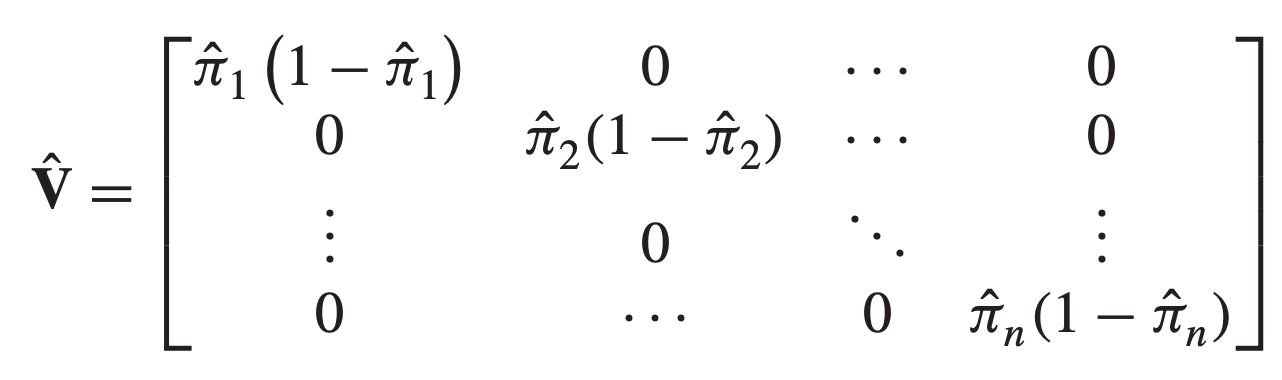
\[\hat{I}(\hat{\beta}) = X^t \hat{V} X\]Where:
Using the notation \(\hat{\pi}_j = h_{\hat{\beta}}(X^{(j)})\) and \(n = n_{pop}\), we get:
The mean of \(\hat{\beta}\) is the estimated value of \(hat{\beta}\).
The test for goodness of fit test the global quality of the model.
The deviance ratio test is based on the ratio of the likelihood of:
The null model is constructed as follow:
\[h_0 = \frac{1}{n_{pop}} \sum_{j=1}^{n_{pop}} \mathrm{1}_{Y^{(j)}=1}\]Its prediction is simply the percentage of individuals of class 1 in the training data.
The deviance ratio statistics is then:
\[D = -2 \ln \frac{L(h_0)}{L(h_\beta)} \sim \chi_{n_{features}}^2\]This is analogous to the Fisher test used in Linear Regression.
In the Deviance ratio test:
Note that the deviance test is normally done using an oracle (called saturated model):
\[D = -2 \ln \frac{L(h_\beta)}{L(h_{\text{oracle}})} \sim \chi_{n_{pop}-(n_{features}+1)}^2\]As this saturated model is generally unknown, the test is modified to represent the gain in deviance of the fitted model vs a null model \(D_{fitted} - D_{null}\). Using the properties of the \(\ln\) function we can find the deviance ratio test as presented above.
The number of degrees of liberty of the \(chi^2\) distribution is the number of features of the model in the denominator minus the number of features of the model in the numerator.
See:
In logistic regression analysis, there is no equivalence of the \(R^2\) of linear regression but different measures exist:
Deviance ratio test can be applied to a model using only one feature. In this case the fitted model only uses this feature. The test is then done similarly than in the ‘Goodness of fit’ deviance ratio test:
\[D = -2 \ln \frac{L(h_0)} {L(h_{\beta_i})} \sim \chi_1^2\]The Wald test assesses the contribution of individual predictors in a given model. The Wald statistic for \(\beta_i\) is:
\[W_i = \frac{\beta_i^2}{\sigma_{\beta_i}^2} \sim \chi_1^2\]It is also possible to test the vector of \(\beta\):
\[W = \beta^t \Sigma_\beta^{-1} \beta \sim \chi_{n_{features}}^2\]See:
For multiclass problem, the logistic regression is called multinomial logistic regression.
The idea is to perform on regression for the log odds of each of the \(K\) output class. Hence the model will have a set of parameters \(\beta_{k,i}\) where \(k\) represent the output class and \(i\) the feature.
The inference formula is the following:
\[\begin{eqnarray} P(Y^{(j)}=k) &&= \frac{e^{h_{\beta_k} (X)}}{\sum_{l=1}^K e^{h_{\beta_l} (X)}} \\ &&= \frac{e^{\beta_k^t X}}{\sum_{l=1}^K e^{\beta_l^t X}} \end{eqnarray}\]It can also be expressed using the Softmax function:
\[\begin{eqnarray} P(Y^{(j)}=k) &&= softmax(k; h_{\beta_1}(X), \ldots, h_{\beta_K}(X)) \\ &&= softmax(k; \beta_1^t X, \ldots, \beta_K^t X) \\ &&= \frac{e^{\beta_k^t X}}{\sum_{l=1}^K e^{\beta_l^t X}} \end{eqnarray}\]Hence the \(softmax\) function replaces the \(sigmoid\) function in the multiclass problem.
Maximum likelihood estimation is replaced by MAP (maximum a posteriori) estimation and the optimization is done by algorithms like L-BFGS.
See:
See: