In the regression framework, \(X\) represents the explanatory variables and \(Y\) represents the output that is a continuous variable.
For a given predictor \(h_\beta\), the MSE loss is:
\[L(h_\beta; (X, Y)) = \left(Y - h_\beta(X)\right)^2\]Over the whole dataset it is:
\[L(h_\beta) = \frac{1}{n_{pop}}\sum_{j=1}^{n_{pop}} \left(Y^{(j)} - h_\beta(X^{(j)})\right)^2\]For a given predictor \(h_\beta\), the MAE loss is:
\[L(h_\beta; (X, Y)) = \vert Y - h_\beta(X) \vert\]Over the whole dataset it is:
\[L(h_\beta) = \frac{1}{n_{pop}}\sum_{j=1}^{n_{pop}} \vert Y^{(j)} - h_\beta(X^{(j)}) \vert\]For a given predictor \(h_\beta\), the Huber loss is a loss quatradic for small values and then linear (to avoid being to sensitive to outliers). A value \(\delta\) defines the limit between quadratic and linear.
\[L(h_\beta, \delta; (X, Y)) = \begin{cases} \frac{1}{2}\left(Y - h_\beta(X)\right)^2 && \text{if } \vert Y - h_\beta(X) \vert \lt \delta\\ \delta\left(\vert Y - h_\beta(X) \vert -\frac{1}{2} \delta \right) && \text{otherwise} \end{cases}\]Over the whole dataset it is:
\[L(h_\beta) = \frac{1}{n_{pop}}\sum_{j=1}^{n_{pop}} L(h_\beta, \delta; (X^{(j)}, Y^{(j)}))\]See Sigmoid and Softmax to see how to obtain classification outputs.
Cross Entropy is a measure of similarity between two probability distributions. When we talk about Cross Entropy loss it is just the Cross Entropy multiplied by -1 to transform it into a loss. In learning, we compare the unknown true probability distribution \(p\) to the estimated probability distribution \(h_\beta\).
For one \(X\) we get:
\[L(h_\beta, p; (X, Y)) = - \sum_{i=1}^{n_{class}} p(Y=i) \log\left(h_\beta^{(i)}\left(X\right)\right)\]Where:
So over the whole dataset we get:
\[l(\beta) = - \sum_{j=1}^{n_{pop}} L(h_\beta, p; (X^{(j)}, Y^{(j)})) = \sum_{j=1}^{n_{pop}} \sum_{i=1}^{n_{class}} p(Y^{(j)}=i) \log\left(h_\beta^{(i)}\left(X^{(j)}\right)\right)\]The general definition of cross entropy is applied to two distributions:
The formula is:
Note that Cross Entropy is not symmetric.
Binary cross entropy loss is a loss function for binary classification.
In the binary case, only two classes are considered: \(p(Y=0)\) and \(p(Y=1)\) and
\[p(Y=0) = 1 - p(Y=1)\]Also note that for label \(Y\), \(Y = P(Y=1)\).
Over the whole dataset we obtain:
\[l(\beta) = \sum_{j=1}^{n_{pop}} Y^{(j)} \log(h_\beta(X^{(j)})) + (1-Y^{(j)}) ( 1-\log( h_\beta( X^{(j)} )))\]Sometimes one might say cross entropy or log loss to refer to binary cross entropy.
In the special case of binary cross entropy, only two classes are considered: \(p(Y=0)\) and \(p(Y=1)\). Also :
\[p(Y=0) = 1 - p(Y=1)\]The formula from cross entropy (multi class cross entropy) can be simplified and the Binary cross entropy loss is for one \(X\):
\[\begin{eqnarray} L(h_\beta, p; (X, Y)) &&= -\left[p(Y=1)\log(h_\beta^{(1)}(X)) + p(Y=0)\log(h_\beta^{(0)}(X))\right]\\ &&= -\left[p(Y=1)\log(h_\beta^{(1)}(X)) + (1-p(Y=1))(1-\log(h_\beta^{(1)}(X)))\right] \\ &&= -\left[Y \log\left(h_\beta(X)\right) + (1-Y) (1-\log\left(h_\beta(X))\right)\right] \end{eqnarray}\]We obtain here the same formula as for the log likelihood in the logistic regression.
Sometimes we refer to this loss without the \(log\) which gives:
\[L(h_\beta, p; (X, Y)) = - \left[h_\beta^{(1)}(X)\right]^{p(Y=1)} + \left[h_\beta^{(0)}(X)\right]^{p(Y=0)}\]The relation between these two formulas is easy to highlight just by applying the log.
Logistic loss / Deviance loss is a loss function for binary classification.
Using the alternative notation \(Y \in \{-1, 1\}\), Logistic loss / Deviance loss are the same as Binary cross entropy loss / Log loss. Let’s show this and in the special cas of logistic regression:
\[h_\beta(X)=g(\beta X)=\frac{1}{1+e^{-\beta X}}\]We can write:
\[\begin{cases} P(Y=1 \vert X; \beta)=\frac{1}{1+e^{-\beta X}}\\ P(Y=0 \vert X; \beta)=1 - \frac{1}{1+e^{-\beta X}}=\frac{e^{-\beta X}}{1+e^{-\beta X}}=\frac{1}{1+e^{\beta X}}\\ \end{cases}\]Remark that the only difference between \(P(Y=1 \vert X; \beta)\) and \(P(Y=0 \vert X; \beta)\) is the sign in the exponential. So using the label \(Y \in \{-1, 1\}\) we can rewrite:
\[P(Y \vert X; \beta) = \frac{1}{1+e^{-Y\beta X}}\]Applying MLE on this we get:
\[\begin{eqnarray} L(\beta) &&= P(Y \vert X; \beta) \\ &&= \prod_{j=1}^{n_{pop}}P(Y^{(j)} \vert X^{(j)}; \beta) \\ &&= \prod_{j=1}^{n_{pop}}\frac{1}{1+e^{-Y^{(j)}\beta X^{(j)}}} \\ \end{eqnarray}\]Applying the log to get log MLE:
\[\begin{eqnarray} l(\beta) &&= \log L(\beta) \\ &&= \log \left[\prod_{j=1}^{n_{pop}}P(Y^{(j)} \vert X^{(j)}; \beta)\right] \\ &&= \sum_{j=1}^{n_{pop}}Y^{(j)} -\log \left(1+e^{-Y^{(j)}\beta X^{(j)}}\right) \end{eqnarray}\]Logistic loss is a loss so we want to minimise and not maximise so we multiply by -1 and we get the loss:
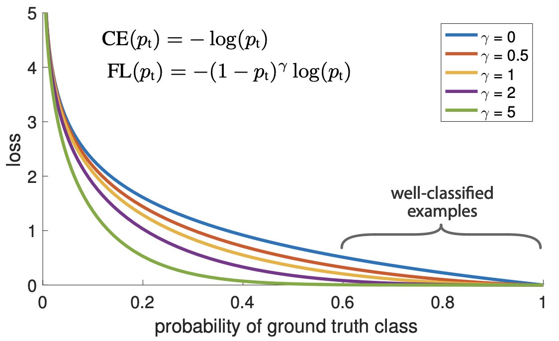
\[L(h_\beta; (X, Y)) = \log \left(1+e^{-Y}\beta X\right)\]Focal loss is a binary classification loss used for unbalanced dataset.
First let’s define \(p_t\) such as:
\[p_t = \begin{cases} h_\beta(X) && \text{if } Y = 1\\ 1-h_\beta(X) && \text{otherwise} \end{cases}\]Using the definition of \(p_t\), the Binary Cross Entropy loss is:
\[L(p_t) = -\log(p_t)\]Here are some visualisation of the focal loss for different \(\gamma\) values and \(\alpha=1\) (and comparison with Binary Cross Entropy):
Exponential loss is:
\[L(h_\beta; (X, Y))=e^{- h_\beta(X) \cdot Y}\]This is the loss used in AdaBoost.
Hinge loss is for binary classification where output \(Y \in \{-1, 1\}\) is:
\[L(h_\beta; (X, Y))=\max(0,1 - h_\beta(X) \cdot Y)\]Different extensions for multi class classification exist such as Crammer and Singer extension:
\[L(h_\beta; (X, Y))=\max(0,1 + \max_{i \neq Y} h_\beta^i(X) - h_\beta^Y(X))\]Where:
This is the loss used in SVM.
See: