Deep Q Network (DQN) is a value based model.
In 2015, Deep Mind developed a new type of Reinforcement Learning model that only took raw pixels as input.
The heart of the model was a Convolutional Neural Network (CNN).
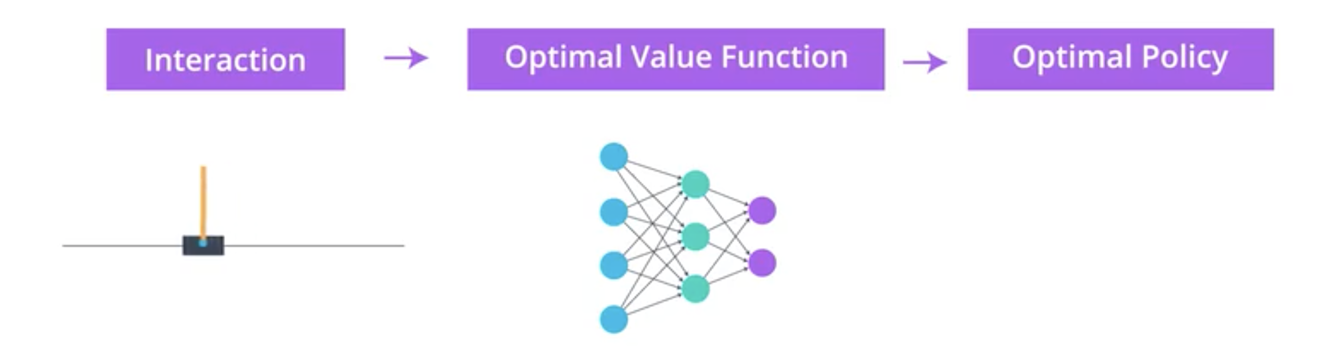
The Deep Q Network (DQN) is still a value based method as it estimates the action value function in order to estimate the policy, hence it can’t deal with actions with continuous spaces:
The update of the parameter is done using a temporal differences method.
The policy is estimated taking the best action ie the action that maximise the futur returns. It is done in a \(\varepsilon\)-greedy fashion:
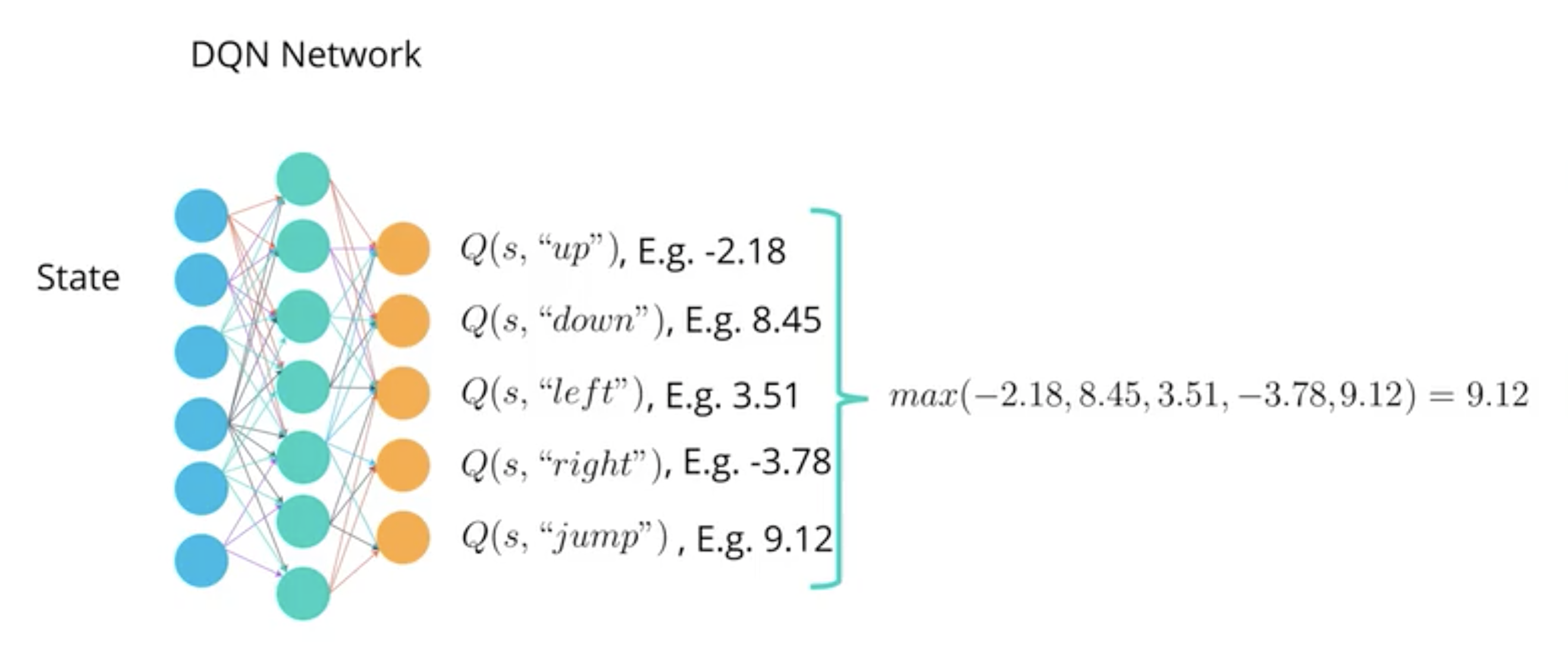
Here the best action is the action “jump”. With \(\varepsilon\)-greedy method, the model would choose the action “jump” with probability \(1-\varepsilon\) and any other action with probability \(\varepsilon\) (\(\varepsilon/(nb_{actions}-1)\)).
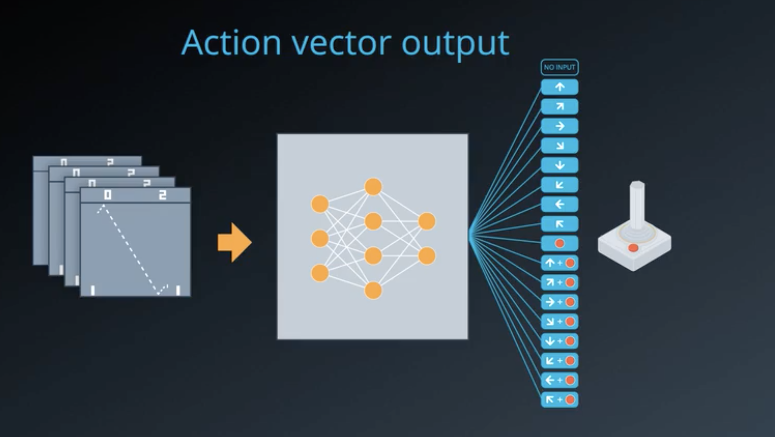
To play pong game the DQN model tooks a sequence of 4 frames as input (4 frames of 84X84 greyscaled pixels) and output the expected return for each action, the best policy is then to choose (in an \(\varepsilon\)-greedy fashion) the action that leads to the best returns:
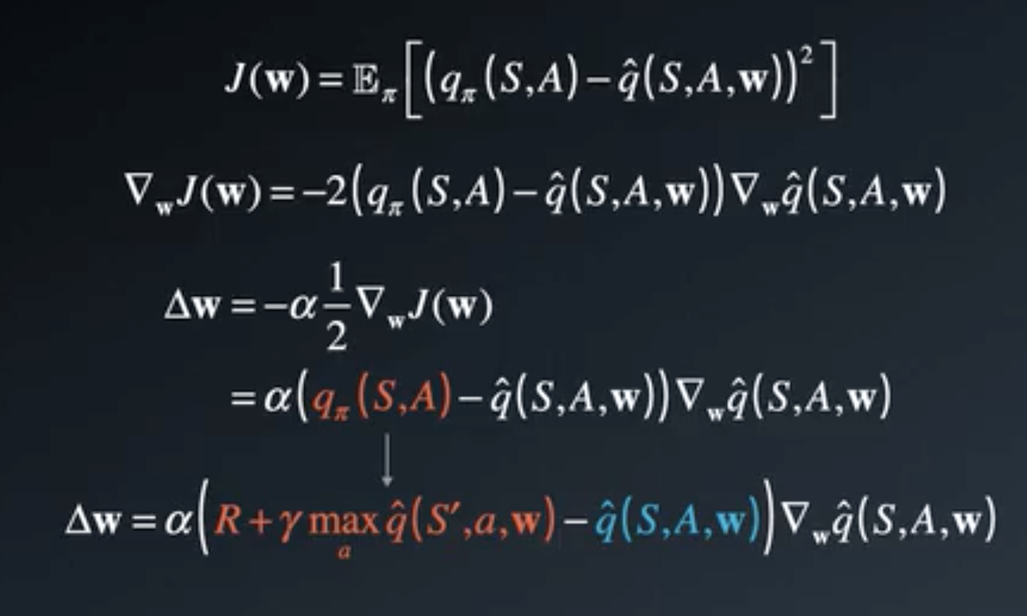
The goal of the DQN is to update its parameters \(w\) to fit the action value function \(q_\pi^*\). The model interacts with the environment and take advantage of the obtained information to update its network.
The update rules is the same as the update rule in temporal differences: the total return \(G_t\) is unobserved and is approximate by the observed reward and the returns of the next state (estimated using our current DQN).
Let \(\Delta(w)\) be the update of the parameters:
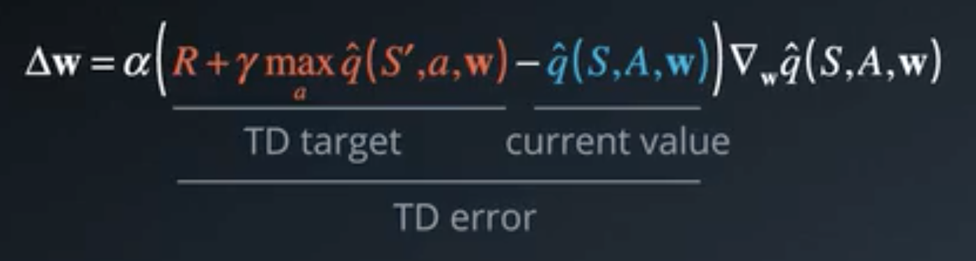
Remark that DQN uses the best action for state \(s'\) like in Sarsamax.
Also remark that this update rule is exactly the result of applying Gradient Descent in order to optimize the Mean Square Error loss between the result of our DQN and \(q_\pi^*\) using the approximation \(R + \gamma \max_{a}\hat{q}(S',a,w)\) of \(q_\pi^*\):
In order to helps the convergence of the network calibration, the DQN uses some tricks.
Experience replay separate the exploration part of the agent from the training part where the model is updated.
An experience is an ensemble of 4 values \(\{S_t, A_t, R_{t+1}, S_{t+1}\}\) that can be used to update the models.
Experience replay uses the current model to interacts with the environment (from a state, choose an action, observe next reward and next states) and stores these interactions in a replay buffer. After a batch of time the model can use this replay buffer to call back the experiences in whatever order to update its parameters. Once the model is updated it returns interacting with the environment to stores new experiences.
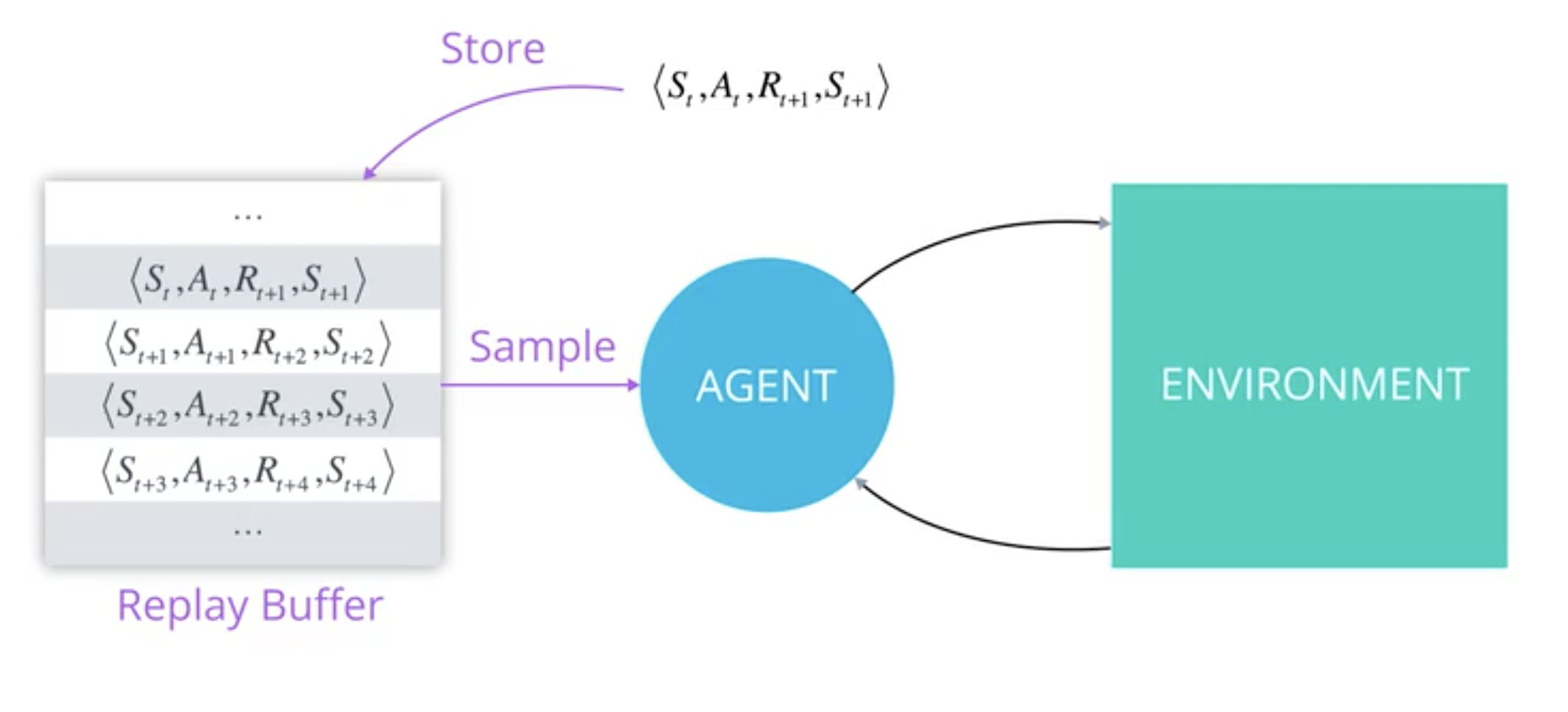
The agent stores the experience and uses it later to update the model.
Here is another visualisation of experience replay. The replay buffer collects different experience and then each mini batch is composed of randomly choosen experiences from replay buffer:
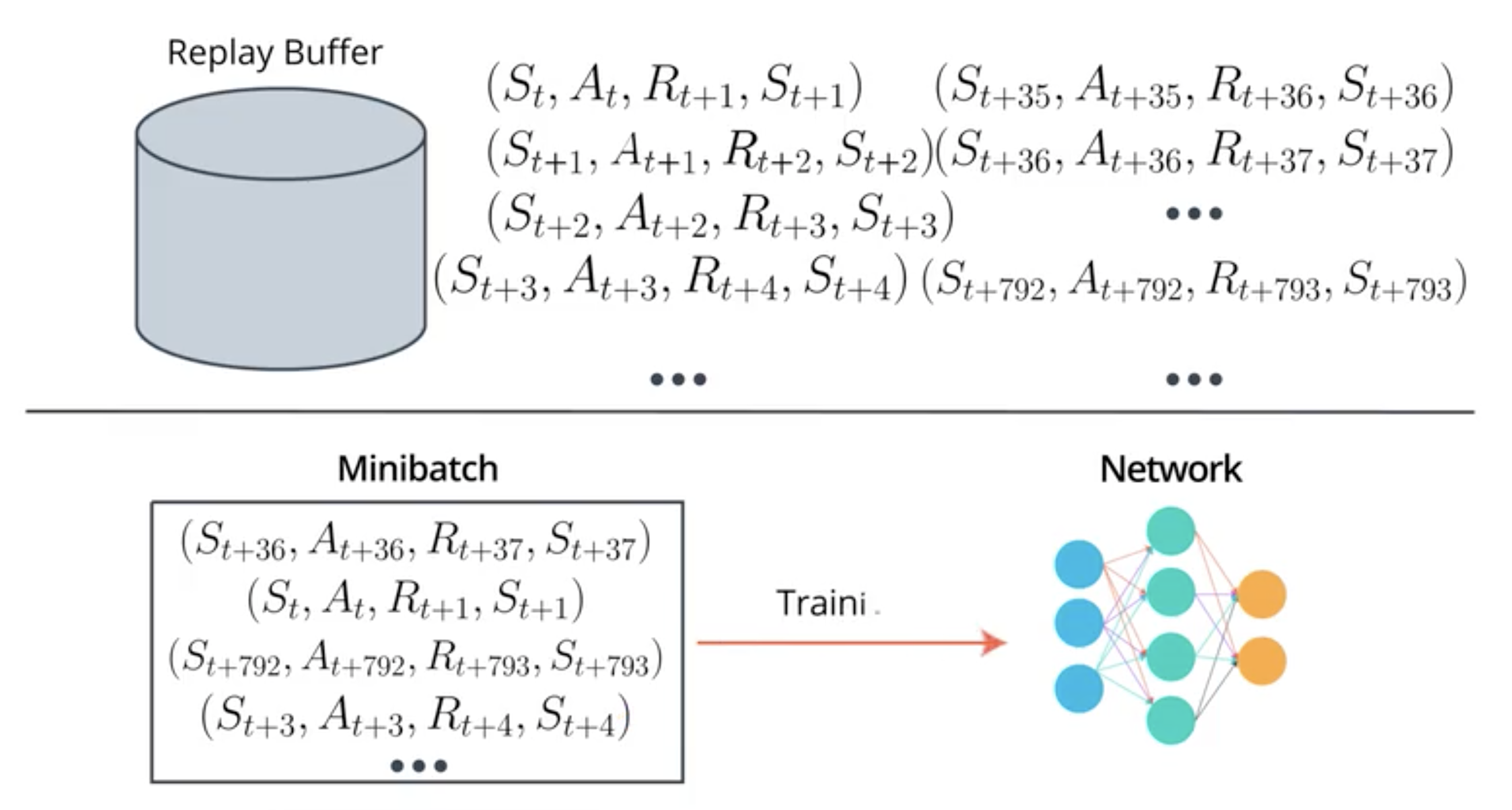
Experience replays avoid to stay stuck in a configuration where one action gave a good reward and hence the agent always choose this action.
Also it transforms the reinforcement learning problem in a series of supervised problems.
It is possible to prioritized the experience replay in order to select the experiences with high error more often in an AdaBoost fashion:
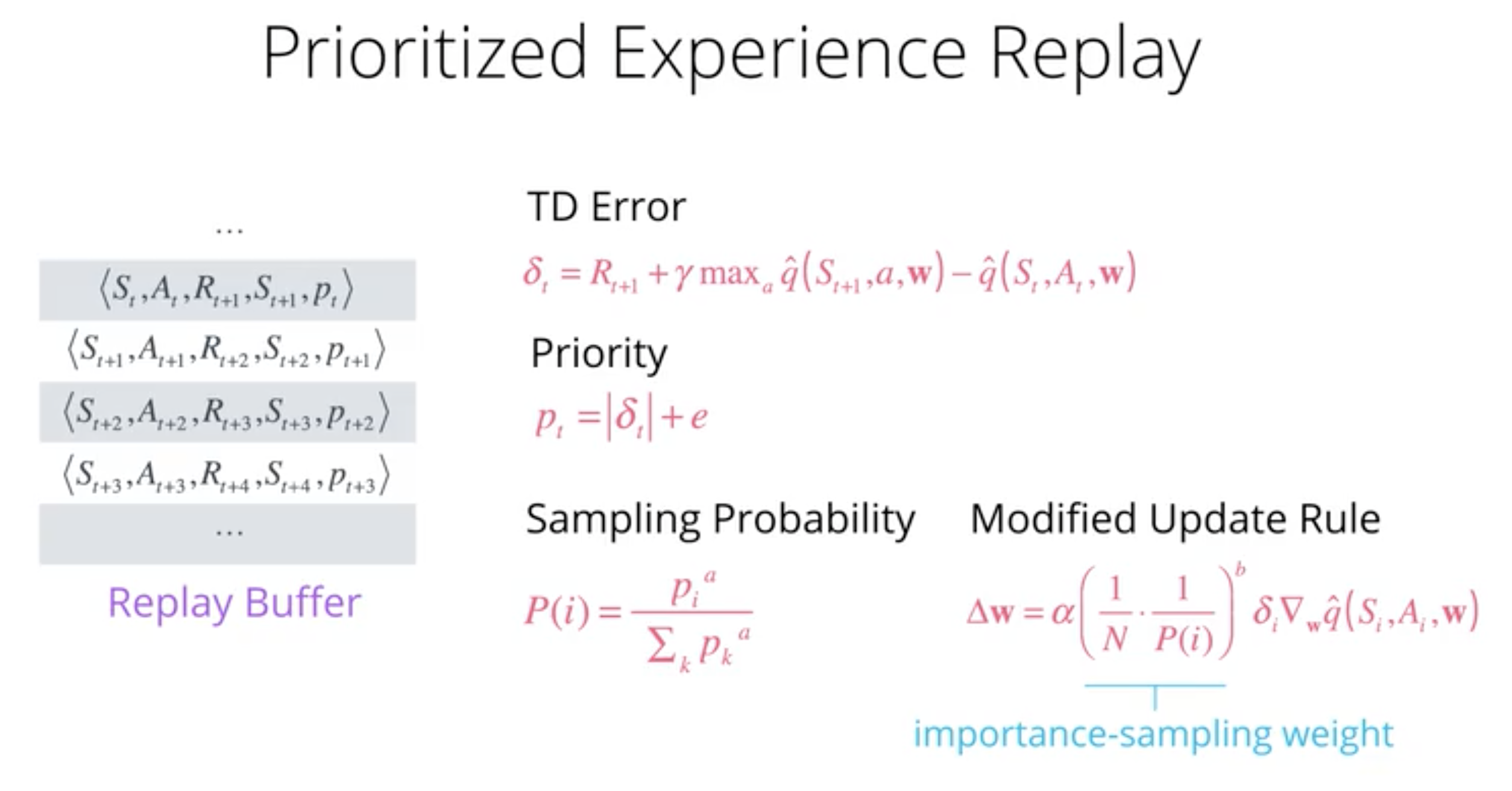
The different steps to use Prioritized Experience replay are:
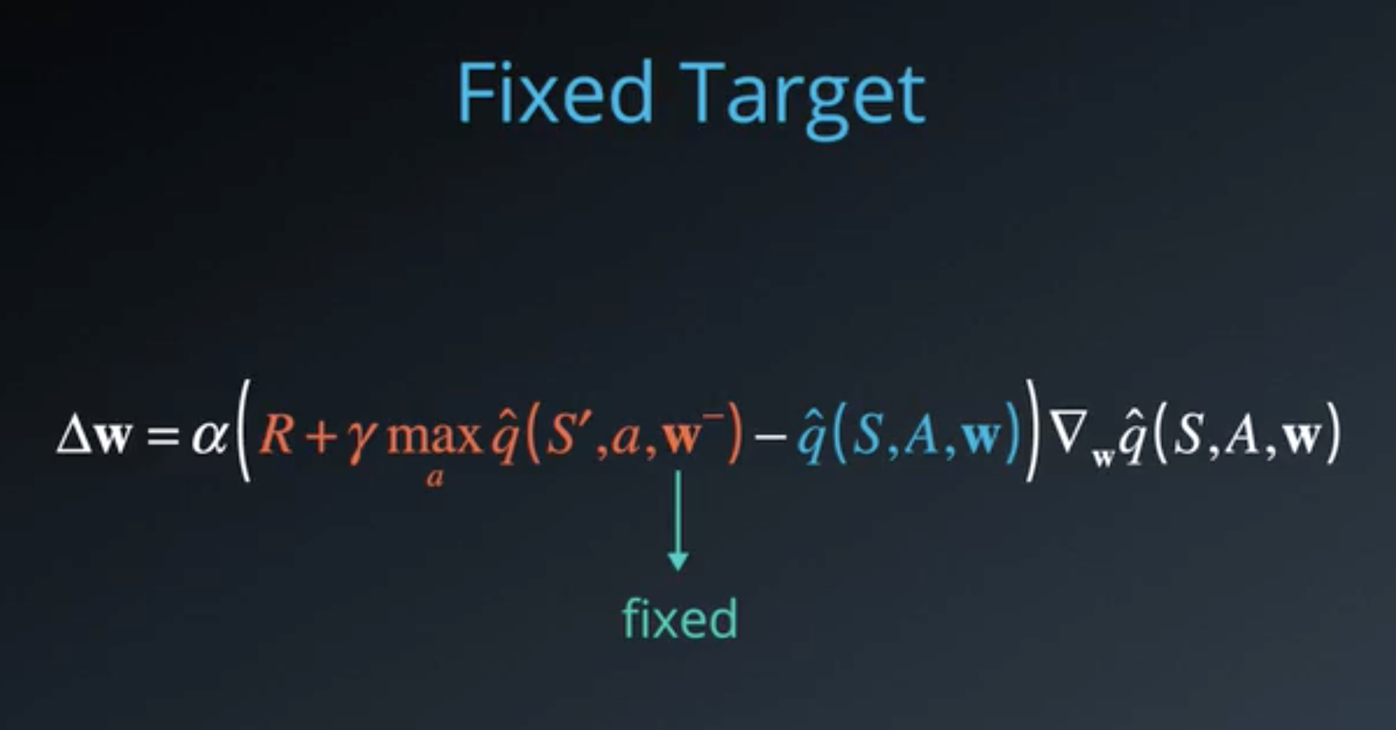
The problem with our update rule is that the objective value (that is an approximation of the true objective function \(q_\pi\)) is dependent on the same variables as the network we want to update. We call this a moving target.
In order to avoid this problem and to fix the target we use the parameters from last iteration in the estimation of the next state/action return:
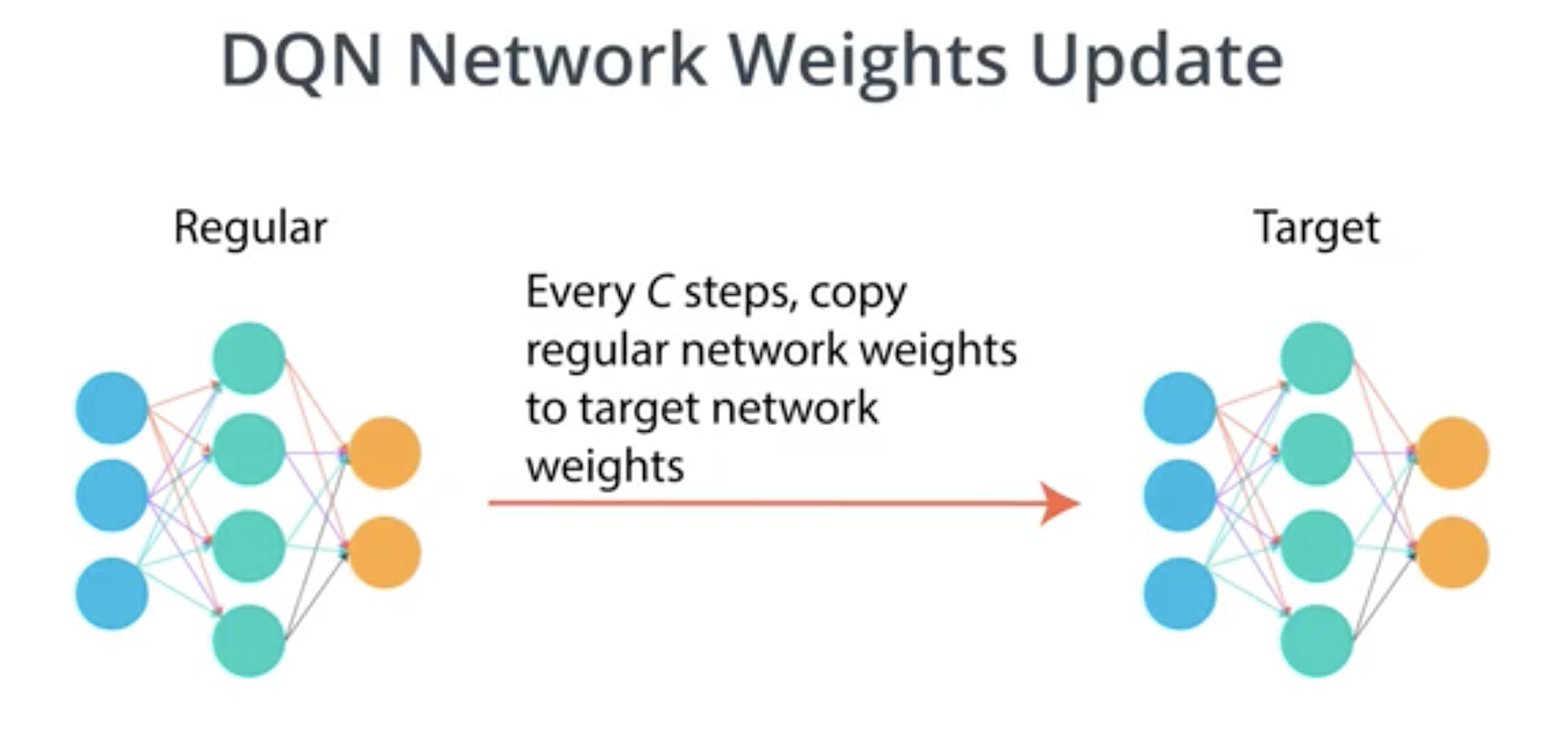
Then DQN maintains two networks, the ‘regular’ network and the ‘target’ network which is a lagged copy of the regular network. It is well reprsented in this image:
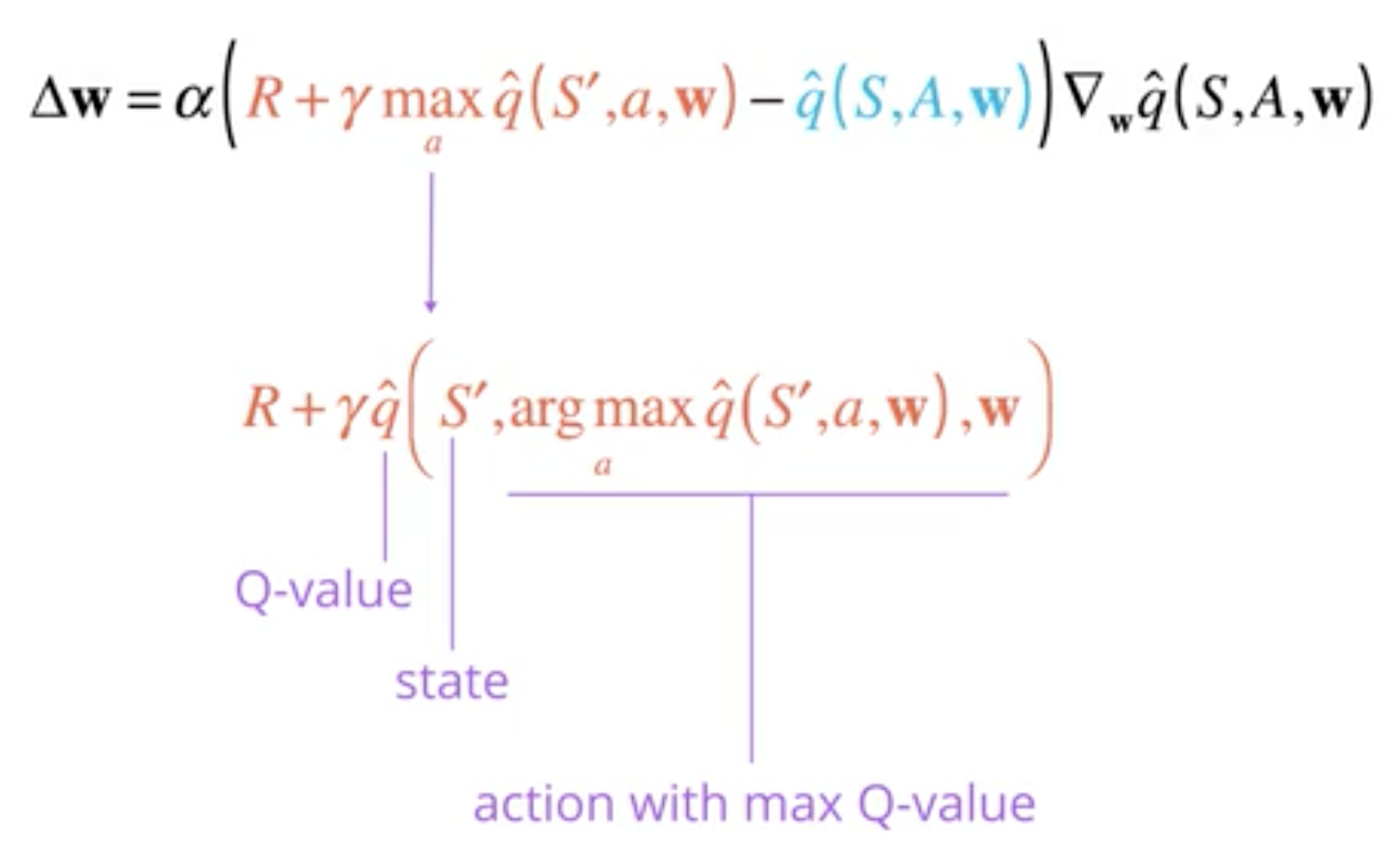
The approximation \(R + \gamma \max_{a}\hat{q}(S',a,w)\) of the true action function \(q_\pi\) over estimates \(q_\pi\). We take the best action possible to make this proxy but the benefits of each action are estimated. By taking the maximum of unstable values we overestimate the true \(q_\pi\).
The idea of Double Q-Learning is to estimate the best action using one network and to compute the associated return using a second network:
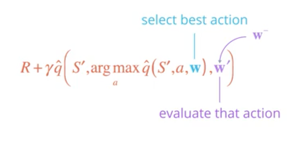
For the DQN model we already keep a second set of parameters \(w^{-}\) in the fixed target.
Hence we evaluate the best action using \(w\) and compute its return using \(w^{-}\):
Dueling Network modifies the structure of the classic DQN to estimate the state value function from one part and defined the action value function as the state value function + an adjustment (an advantage value) coming from the action.
Using this, all actions from a state share a common basis value which seem logical:
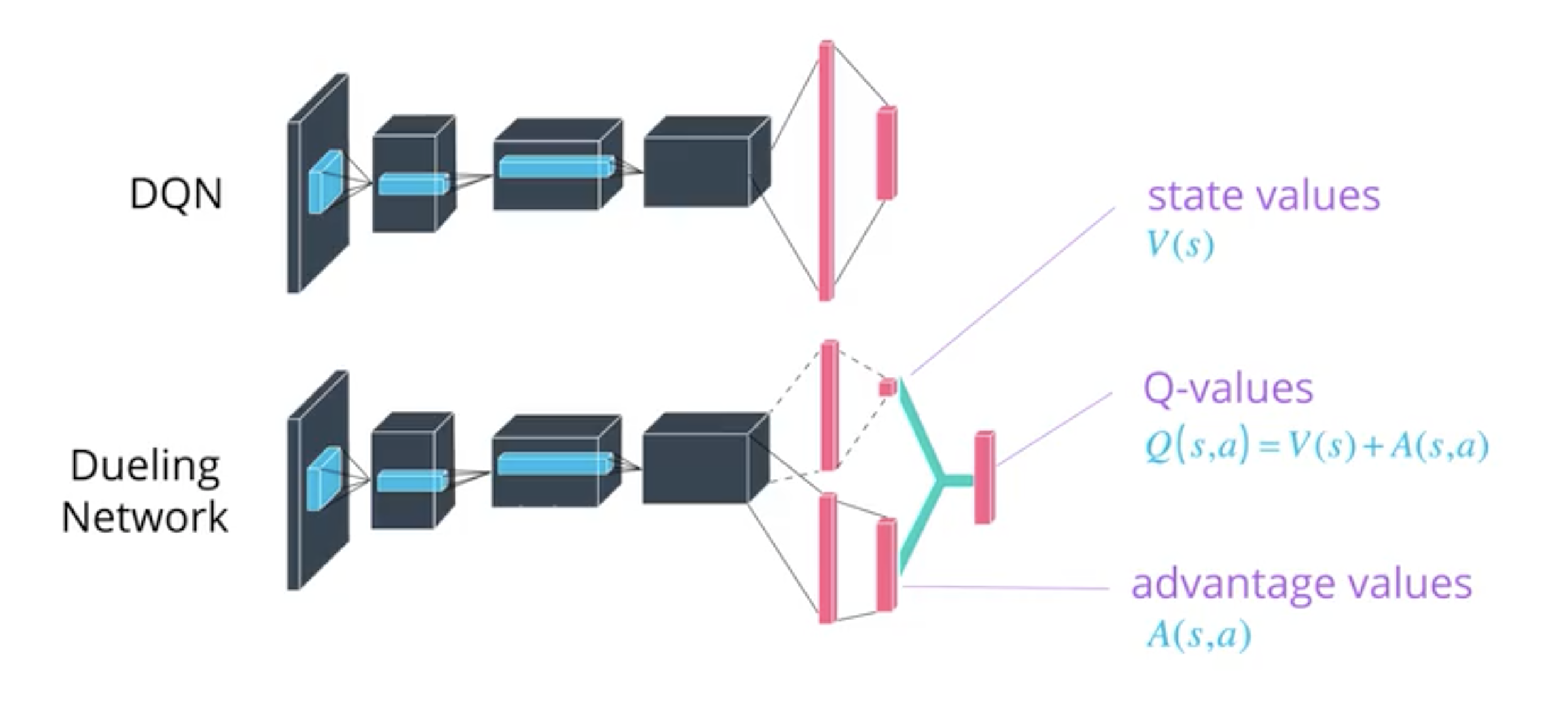
The advantage function \(A_\pi(s,a)\) is the advantage of an action \(a\) with respect to a state \(s\). It is the difference between the action value function \(Q_\pi(s,a)\) and the state value function \(V_\pi(s)\):
\[A_\pi(s,a) = Q_\pi(s,a) - V_\pi(s)\]Equivalently:
\[Q_\pi(s,a) = V_\pi(s) + A_\pi(s,a)\]Which is used in the Dueling Network.
See: