A Convolutional Neural Network or CNN is a type of neural network specifically designed to be applied to images.
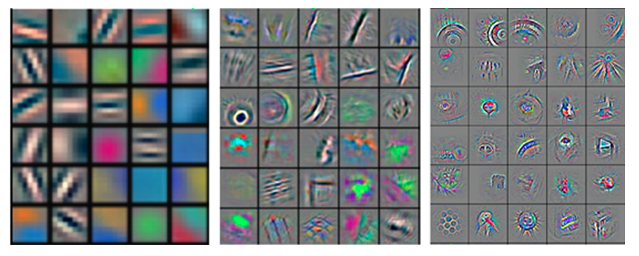
A CNN uses layers of filters made of weights that are designed to extract features from the images. As we go deeper in the model, the features extracted are more and more complex:
The advantages of using a CNN over a classical feed forward neural network for images are:
Convolution is a mathematical operation. CNN uses 2d convolutions.
The mathematical convolution is:
\[(f \ast g)(x)= \int_{-\infty}^{+\infty} f(x-t) g(t) \; \mathrm{d}t = \int_{-\infty }^{+\infty} f(t) g(x-t) \; \mathrm{d}t\]In discrete space it is:
\[(f \ast g)(n)= \sum_{m=-\infty}^{+\infty} f(n-m) g(m) = \sum_{m=-\infty }^{+\infty} f(m) g(n-m)\]CNN uses 2d convolution.
Here is a representation of convolution in dimension 1 of a function applied to itself ie \(f=g\):
In the above example:
\[f(x) = g(x) = \begin{cases} 1 && \text{if } -0.5 \leq x \leq 0.5\\ 0 && \text{otherwise} \end{cases}\]\((f \ast g)(x)\) is not null if:
\[0.5 \leq t \leq 0.5 \text{and} 0.5 \leq x-t \leq 0.5 \; \forall t \in \mathbb{R}\]In this special case, the convolution can be rewrite:
\[(f \ast g)(x) = \int_{-0.5}^{+0.5} f(x-t) \; \mathrm{d}t\]It is easy to see that it is non null for \(-1 \leq x \leq 1\).
See:
A CNN model is a succession of convolution layers, activation functions, pooling and that ends with fully connected layers:
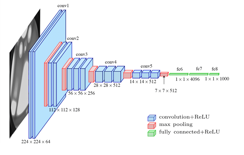
Representation of VGG-16 model.
Some CNN are also encoder decoder. This means that the information of an image is encoded in a smaller dimension and then is decoded to a larger resolution to perform, for example, image segmentation:
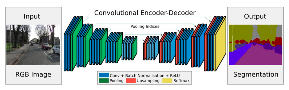
Representation of SegNet.
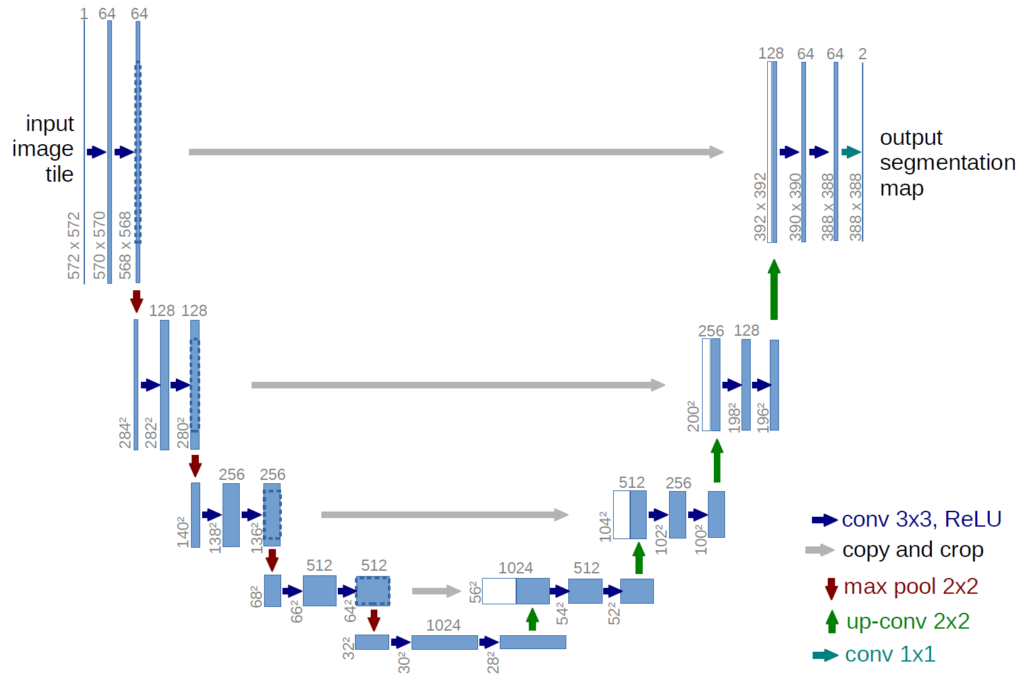
Another (fancier) encoder decoder model is U-Net:
The main blocks of a CNN are convolutional layers.
Convolutional layers apply \(K\) convolutional filters (also called kernels) on the output of the precedent layer (or directly on the input for the first convolutional layer).
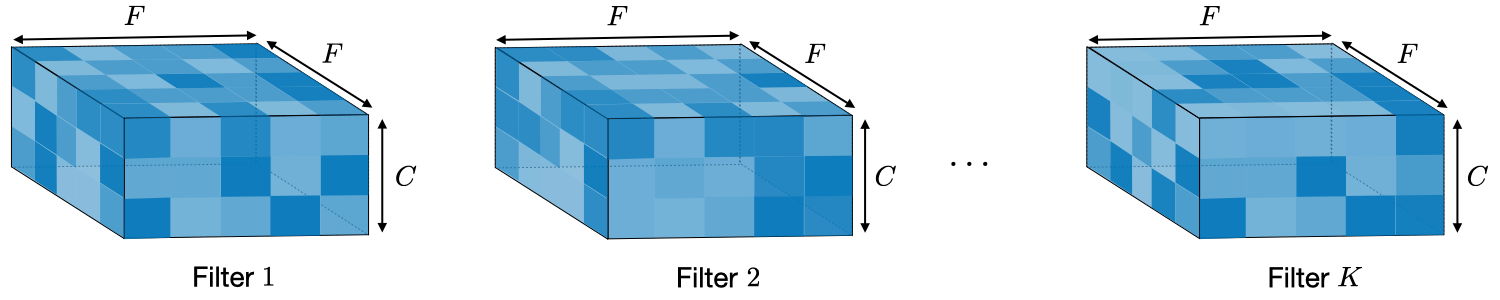
Convolutional filters are of size \((F \times F \times C)\) where \(F\) is the height and width of the filter and \(C\) the number of output channels from previous layers (an RGB image has 3 channels).
Here is a representation of a layer of \(K\) filters of size \(F \times F \times C\).
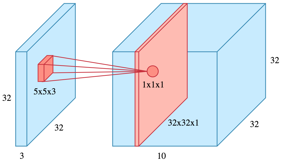
And here is a representation of a filter (in red) of size \((5 \times 5 \times 3)\) (3 being the number of channel of the input - or precedent layer) applied to an input (input data or output of precedent layer) of size \((32 \times 32 \times 3)\):
Generally, a convolutional filter is of size \((3 \times 3)\) as a serie of \((3 \times 3)\) convolutional layer can achieve the same receptive field as larger convolution filters.
For example a stack of 3 layers of \(C\) filters of size \((3 \times 3 \times C)\) has the same receptive fields as a single layer of \(C\) filter of size \((7 \times 7 \times C)\). However the first setup has \(3 \times (C \times (3 \times 3 \times C)) = 27C^2\) parameters and the second setup has \((C \times (7 \times 7 \times C)) = 49C^2\) parameters (see CS231n course on CNN, paragraph on Layer Patterns).
A \((F \times F)\) filter applied to a \((H \times H)\) image will decrease its size. The output size will be: \(\left[(H-F+1) \times (H-F+1)\right]\).
The receptive field at layer \(k\) is the area denoted \(R_k \times R_k\) of the input that each pixel of the \(k\)-th activation map can ‘see’.
Here is a visual representation of the receptive field:
More information on receptive field on CS230n cheatsheet on CNN.
Here is a visual representation of a filter of size \((3 \times 3 \times 1)\) applied to an input image of \(0\) and \(1\) of size \((5 \times 5 \times 1)\):
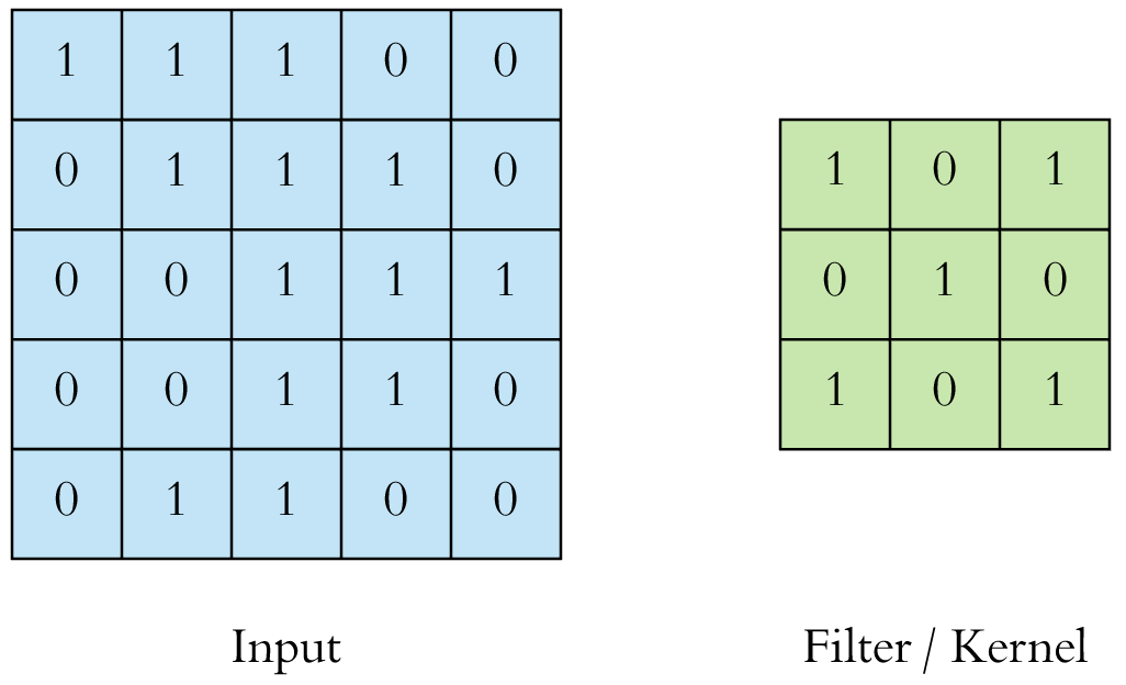
The kernel is applied to every possible position:
Note that the size in decreased by the application of a filter.
Naturally a convolutional filter moves by 1 pixel at a time but it can move 2 pixels by 2 pixels or by any number of pixel. This is called the stride.
Here is a \((3 \times 3)\) filter with stride 1:
Here is a \(3 \times 3\) filter with stride 2:
A \((F \times F)\) filter with stride \(S\) applied to a \((H \times H)\) image will decrease its size. The output size will be: \(\left[\left(\frac{H-F}{S}+1\right) \times \left(\frac{H-F}{S}+1\right)\right]\).
Padding consist in adding null pixels around the input in order to not decrease (or limit) the size of the input.
Here is a \(3 \times 3\) filter with stride 1 and padding 1:
The output size of a \(F \times F\) filter with stride \(S\) and padding \(P\) applied to a \(H \times H\) image will be: \(\left[\left(\frac{H-F+2P}{S}+1\right) \times \left(\frac{H-F+2P}{S}+1\right)\right]\).
Pooling is an operation that reduce the dimension of the input. The goal of pooling is to reduce the number of parameters of the model which both shorten the training time and combat overfitting.
The most common pooling is max pooling which only keep the most import (greater) value in an area:
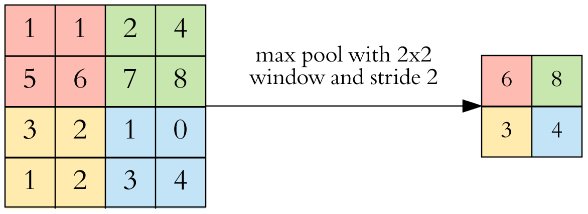
Here the max pooling operation is of size \((2 \times 2)\) with stride 2. This is the commonly used max pooling.
Instead of max pooling one can use average pooling which average the features of the area.
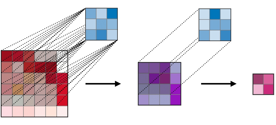
Here is a representation of dimension reduction done by max pooling operation:
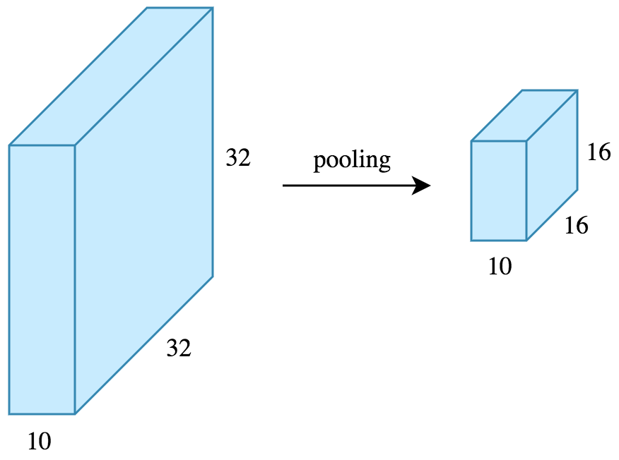
See: