XGBoost is a special type of gradient descent methods that adds some improvment of the base Gradient Descent algorithm.
The first trick used by XGBoost is to use the Newton’s method ie to not use the first order approximation in the Taylor expansion but the second order:
\[\begin{eqnarray} L(Y, T_{k-1}(X)+t(X)) &&= L(Y, T_{k-1}(X)) + t(X) \frac{d}{dT_{k-1}(X)}L(Y, T_{k-1}(X)) + \frac{1}{2} t(X)^2 \frac{d^2}{d^2T_{k-1}(X)}L(Y, T_{k-1}(X)) + o(t(X)^2) \\ &&= L(Y, T_{k-1}(X)) + t(X) g_{k-1} + \frac{1}{2} t(X)^2 h_{k-1} + o(t(X)^2) \end{eqnarray}\]Where:
We can no longer use gradient descent to find the find our update rule by fining \(t\) that best fits (it would require finding a learner that fit himself plus something).
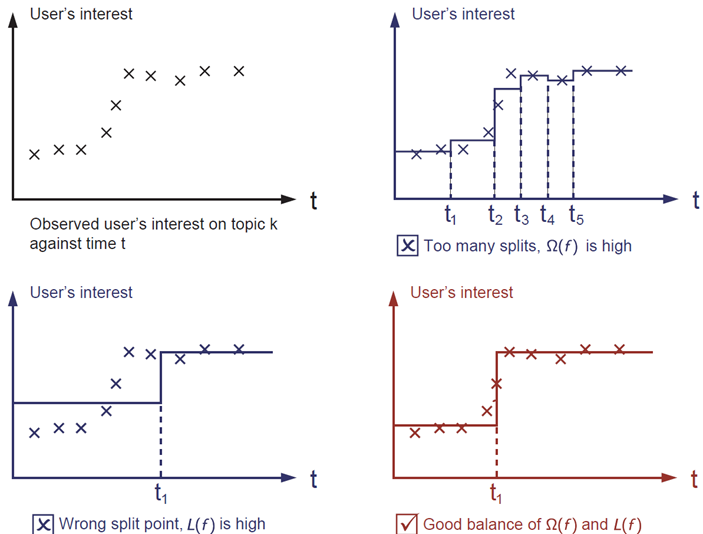
XGBoost also adds a regularization on the structures of its trees. It penalizes the leafs’ number and the leaf values. It allows to limit overfitting:
Assume:
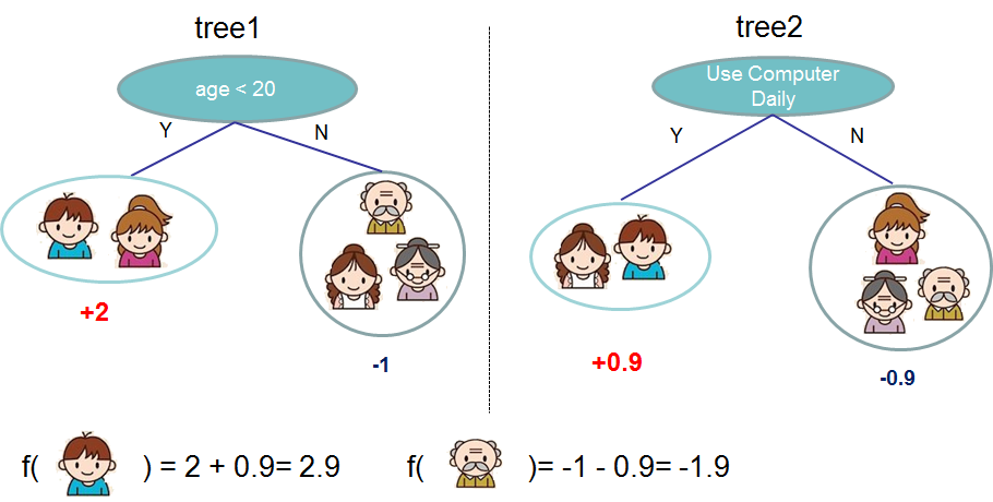
We are here in the case of a regression tree and not a decision tree. Unlike decision trees, each regression tree contains a continuous score on each of the leaf, represented here by \(w_m\):
Then, the regularization for tree \(t\) is:
\[\Omega(t)=\gamma \left(\text{Leafs}\right) + \frac{1}{2}\lambda \Vert w \Vert_2^2\]The regularization limits the numbers of leafs and the weight associated to tree \(t\) to avoid overfitting. Similar regularization can be created for decision trees.
So \(L(Y, T_{k-1}(X)+t(X))\) becomes:
\[\begin{eqnarray} L(Y, T_{k-1}(X)+t(X)) &&= \left[L(Y, T_{k-1}(X))\right] + \left[t(X) g_{k-1}\right] + \left[\frac{1}{2} t(X)^2 h_{k-1}\right] + \gamma \left(\Omega(t)\right) + o\left(t(X)^2\right) \\ &&= \left[L(Y, T_{k-1}(X))\right] + \left[t(X) g_{k-1}\right] + \left[\frac{1}{2} t(X)^2 h_{k-1}\right] + \left[\gamma \left(\text{Leafs}\right) + \frac{1}{2}\lambda \Vert w \Vert_2^2\right] + o\left(t(X)^2\right) \end{eqnarray}\]Given the function loss \(L(Y, T_{k-1}(X)+t(X))\) with the regularization and approximated using Newton’s method, XGBoost finds a quick way to estimate the loss for a given \(t\) and for every splits.
Let’s compute the loss for one \(t\), for every \(X^{(j)}\) (every sample). We can ignore \(L(Y, T_{k-1}(X))\) and \(o(t(X)^2)\)) (as the first the equivalent for all \(t\) and the second is negligeable). Let’s also call it \(L(t)\) as our variable is \(t\).
\[\begin{eqnarray} L(t) &&= \sum_{j=1}^{n_{pop}} L(Y, T_{k-1}(X^{(j)})+t(X^{(j)})) \\ &&= \sum_{j=1}^{n_{pop}} \left[t\left(X^{(j)}\right) g_{k-1} + \frac{1}{2} t\left(X^{(j)}\right)^2 h_{k-1} + \gamma \left(\text{Leafs}\right) + \frac{1}{2}\lambda \sum_{m=1}^{L} w_m^2 \right] \\ &&= \sum_{m=1}^{\text{Leafs}} \left[ \left(\sum_{j \in l_m} g_{k-1}\right) w_m + \frac{1}{2} \left(\sum_{j \in l_m} h_{k-1} + \lambda \right) w_m^2 \right] + \gamma \left(\text{Leafs}\right) \end{eqnarray}\]Line 2 to line 3 uses that, for a given leaf \(m\) of tree \(t\), for an individual \(X^{(j)}\) that belongs to this leaf, we can replace \(t(X^{(j)})\) by \(w_m\) and \(t\left(X^{(j)}\right)^2\) by \(w_m^2\) as the value that \(t\) will associate to \(X^{(j)}\) is \(w_m\) (each element of a leaf will be associated to the same value).\
All the individuals of a given leaf \(m\) share the same weight \(w_m\) and we can therefore factorize the individual of a leaf by \(w_m\).
We transform the sum over all element in two nested sums:
Now we can compute the optimal value for every \(w_m\) and compute the loss for \(t\).
Let’s differentiate wrt \(w_m\) and set to 0 to find a minimum:
\[\frac{d}{dw_m} L(Y, T_{k-1}+t) = \sum_{j \in l_m} g_{k-1} + w_m \left(\sum_{j \in l_m} h_{k-1} + \lambda \right)\]Setting the loss to 0 and resolving for \(w_m\), we obtain:
\[w_m^* = - \frac{ \sum_{j \in l_m} g_{k-1} } { \sum_{j \in l_m} h_{k-1} + \lambda }\]\(w_m^*\) is the weight that will be use for individuals of leaf \(m\) in the tree \(t\). It is simply computed as the derivative of the loss \(L\) with respect to the current strong learner \(T\) over the Hessian (second derivative) of the loss \(L\) with respect to the current strong learner \(T\). It is a direct application of Newton’s method.
Replacing the \(w_m\) by this obtained value gives the total loss for \(t\):
\[\begin{eqnarray} L(t) &&= \sum_{m=1}^{L} \left[ \left(\sum_{j \in l_m} g_{k-1}\right) \left(- \frac{ \sum_{j \in l_m} g_{k-1} } { \sum_{j \in l_m} h_{k-1} + \lambda }\right) + \frac{1}{2} \left(\sum_{j \in l_m} h_{k-1} + \lambda \right) \left(- \frac{ \sum_{j \in l_m} g_{k-1} } { \sum_{j \in l_m} h_{k-1} + \lambda }\right)^2 \right] + \gamma L \\ && = \sum_{m=1}^{L} \left[ -\frac{ \left(\sum_{j \in l_m} g_{k-1}\right)^2 } { \sum_{j \in l_m} h_{k-1} + \lambda } + \frac{1}{2} (\frac{ \left(\sum_{j \in l_m} h_{k-1} + \lambda \right) \left(\sum_{j \in l_m} g_{k-1}\right)^2 } { \left(\sum_{j \in l_m} h_{k-1} + \lambda\right)^2} \right] + \gamma L \\ &&=\sum_{m=1}^{L} \left[ -\frac{ \left(\sum_{j \in l_m} g_{k-1}\right)^2 } { \sum_{j \in l_m} h_{k-1} + \lambda } + \frac{1}{2} \frac{ \left(\sum_{j \in l_m} g_{k-1}\right)^2 } { \sum_{j \in l_m} h_{k-1} + \lambda } \right] + \gamma L \\ &&= -\frac{1}{2} \sum_{m=1}^{L} \frac{ \left(\sum_{j \in l_m} g_{k-1}\right)^2 } { \sum_{j \in l_m} h_{k-1} + \lambda } + \gamma L \\ \end{eqnarray}\]This loss can be used as a scoring function to measure the quality of a tree. It can be computed for any loss function for which we can compute its first and second derivatives \(g\) and \(h\).
Note that the \(g_{k-1}\) and \(h_{k-1}\) are common for each tree and each split and only require to be computed once.
Once \(g_{k-1}\) and \(h_{k-1}\), the best tree is easily estimated as:
Gradient Boosting and XBoost are sequential models. The precedent step needs to be known in order to estimate the next weak learner.
However for the estimation of a given weak learner during the process and using the precedent formula, all the computation can be parallelized. Hence finding the best tree at each step is very fast.
XGBoost accepts in its implementation stochastic gradient descent which allows to not compute the loss over the whole dataset everytime and can hence reduce the computation time.
See:
For classification and using the cross entropy loss, the output of our strong learner \(T_{k-1}\) is a sum of Bernoulli variable. So we need to rescale them between 0 and 1 which mean applied the sigmoid function.
This must be taken into account when compute the derivative \(g_{k-1}\) and second derivative \(h_{k-1}\). Chain rule must be used as derivative is compute with respect to \(\hat{Y_{k-1}}\) being a sum of outputs of each tree in \(T_{k-1}\).
The loss function is hence:
\[L=Y \log (\sigma(\hat{Y_{k-1}})) + (1-Y) \log (\sigma(1-\hat{Y_{k-1}}))\]Where:
See:
See: