Revision

Back to Machine Learning

Definition

OPTICS (for Ordering points to identify the clustering structure is a density based clustering) is a clustering method similar to DBSCAN.

The main difference between DBSCAN and OPTICS is that OPTICS does not require an hyperparameter \(\varepsilon\). It still requires an hyperparameter \(min_{points}\). It also used a optional \(max_\varepsilon\) hyperparameter.

Notation

Two data points \(p\) and \(q\) are considered neighbours if \(D(p, q) \lt \varepsilon\) where \(D\) is a given distance measure (euclidian distance for example),
A point \(p\) is a core point if at least \(min_{points}\) neighbours, ie \(min_{points}\) points which are within a distance \(\varepsilon\) of it (including \(p\)),
A point \(q\) is directly reachable from \(p\) if point \(q\) is within distance \(\varepsilon\) from core point \(p\). Points are only said to be directly reachable from core points,
A point \(q\) is reachable from \(p\) if there is a path \(p_1, \ldots, p_n\) with \(p_1 = p\) and \(p_n = q\), where each \(p_{i+1}\) is directly reachable from \(p_i\). Note that this implies that the initial point and all points on the path must be core points, with the possible exception of \(q\),
\(N_{\varepsilon}(p)\) is the set of neighbours of \(p\),
\(min_{distance}(p)\) is the distance from \(p\) to its \(min_{points}\) neighbour,
\(core-distance_{\varepsilon, min_{points}}(p)\) is the distance between \(p\) and its \(min_{points}\) neighbour if \(p\) has \(min_{points}\) neighbours otherwise it is undefined,
\(reachability-distance_{\varepsilon, min_{points}}(p, q)\) is the smallest distance such as \(p\) would be reachable from \(q\) and \(q\) would be a core point wrt to this distance.

\[\text{core-distance}_{\varepsilon, min_{points}}(p) = \begin{cases} Undefined && \text{if } \vert N_{\varepsilon}(p) \vert \lt min_{points}\\ min_{distance}(p) && \text{otherwise} \end{cases}\]

\[\text{reachability-distance}_{\varepsilon, min_{points}}(p, q) = \begin{cases} Undefined && \text{if } \vert N_{\varepsilon}(q) \vert \lt min_{points}\\ \max(\text{core-distance}_{\varepsilon, min_{points}}(q), \; D(p,q)) && \text{otherwise} \end{cases}\]

Note that the \(\text{reachability-distance}\) is not symmetric.

Idea of the algorithm

Using the hyperparameter \(min_{points}\) and the optional hyperparameter \(max_\varepsilon\), OPTICS will create for each point \(p\) a reachability-distance matrix.

If \(max_\varepsilon\) is not defined by the user its default value is \(\infty\). In this setup, every point will have a core-distance and reachability-distance to every points defined. Otherwise some points will have \(undefined\) distances.

Once the reachability-distance matrix is defined, a reachability plot is created. The reachability plot has in \(x\)-axis the points and in \(y\)-axis their reachability distance to the closest point.

The reachability plot is ordered and created incrementaly: for each current point the algorithm selects the next point as the point with minimum reachability-distance to the current point (initialisation is random).

Reachability plot

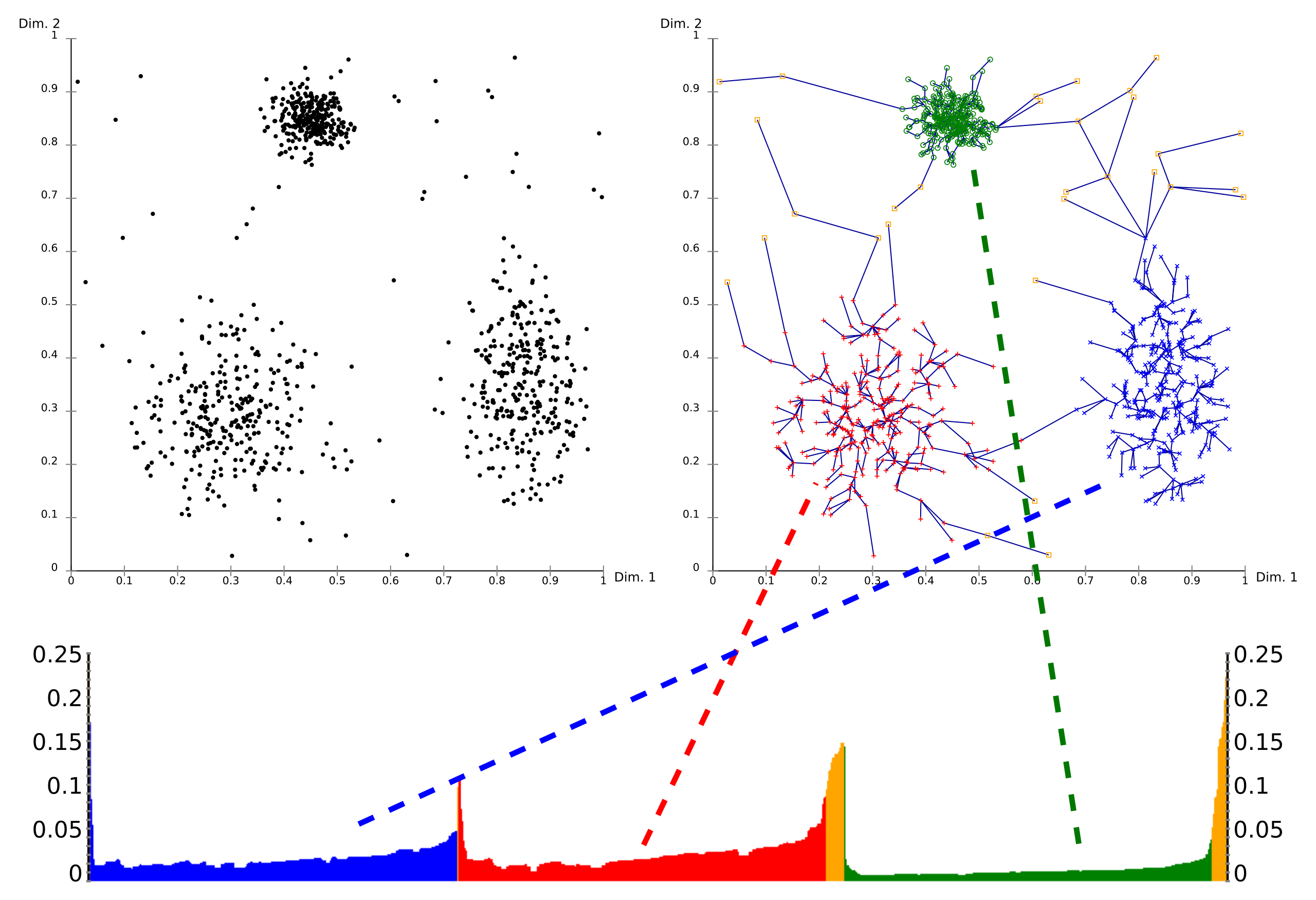
Here is a visualisation of reachability plot:

Using a reachability-plot (a special kind of dendrogram), the hierarchical structure of the clusters can be obtained easily. It is a 2D plot, with the ordering of the points as processed by OPTICS on the x-axis and the reachability distance on the y-axis. Since points belonging to a cluster have a low reachability distance to their nearest neighbor, the clusters show up as valleys in the reachability plot. The deeper the valley, the denser the cluster.

The image above illustrates this concept. In its upper left area, a synthetic example data set is shown. The upper right part visualizes the spanning tree produced by OPTICS, and the lower part shows the reachability plot as computed by OPTICS. Colors in this plot are labels, and not computed by the algorithm; but it is well visible how the valleys in the plot correspond to the clusters in above data set. The yellow points in this image are considered noise, and no valley is found in their reachability plot. They are usually not assigned to clusters, except the omnipresent “all data” cluster in a hierarchical result. From OPTICS Wikipedia page.

Selection of clusters

Extracting clusters from this plot can be done manually by selecting a range on the x-axis after visual inspection, by selecting a threshold on the y-axis (the result is then similar to a DBSCAN clustering result with the same \(\varepsilon\) and \(min_{points}\) parameters; here a value of 0.1 may yield good results), or by different algorithms that try to detect the valleys by steepness, knee detection, or local maxima. From OPTICS Wikipedia page.

Algorithms for cluster extraction are Xi and DBSCAN (see OPTICS on Scikit-Learn).

Pros and cons

Pros

Can cluster different structure shape,
Average complexity \(O(nlog(n))\) if \(max_\varepsilon\) is well selected,
Worts complexity of \(O(n^2)\) if \(max_\varepsilon \lt \max{p,q}D(p,q)\),
Automatically selects the number of clusters (or can be done manually),
Great visualisations,
Not sensitive to hyperparameters (see the different reachability plots from OPTICS: Ordering Points To Identify the Clustering Structure by M Ankerst, M M Breunig, H-P Kriegel and J Sander).

Resources

See: