Revision

Back to Machine Learning

Supervised Metrics

Regression

\(R^2\): Coefficient of determination

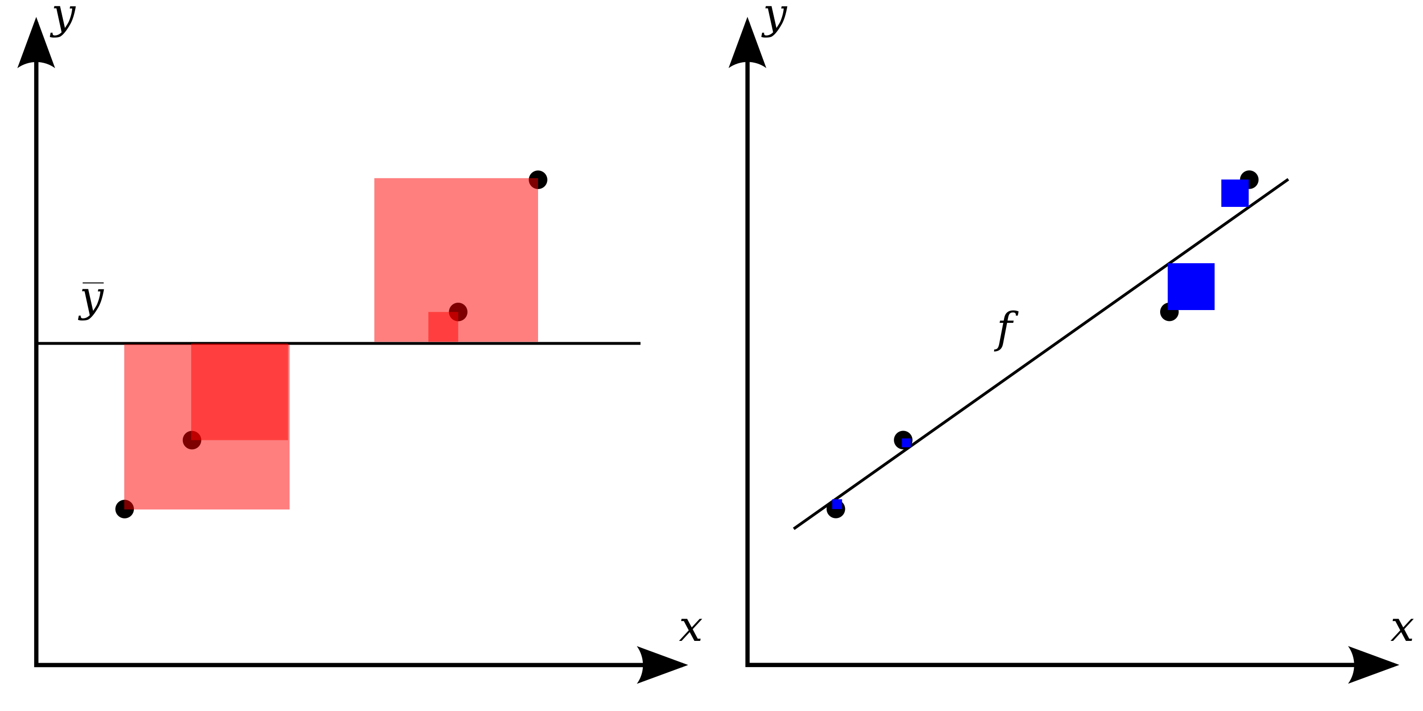
In statistics, the coefficient of determination, denoted \(R^2\) or \(r^2\) is the proportion of the variation in the observed variable (y) that is predictable from the explanatory variables (X). It is a performance metric for linear regression.

Formula

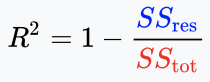
For given predictions \(\hat{y}_i\) and true labels \(y_i\), the \(R^2\) is:

\[R^2=1-\frac{SS_{Residual}}{SS_{Total}}=\frac{SS_{Explained}}{SS_{Total}}\]

Where:

\(SS_{Total}=\sum_{i=1}^n\left(y_i - \bar{y}\right)^2\) represents the total variance of \(y\),
\(SS_{Explained}=\sum_{i=1}^n\left(\hat{y}_i - \bar{y}\right)^2\) represents the variance explained by the estimators \(\hat{y}\),
\(SS_{Residual}=\sum_{i=1}^n\left(y_i - \hat{y}_i\right)^2\) represents the remaining variance, unexplained by the model.

And law of total variance: \(SS_{Total}=SS_{Explained}+SS_{Residual}\).

The following graphics from Wikipedia shows a visual interpretation:

Resources

See:

Coefficient of determination on Wikipedia

Root Mean Square Error

For given predictions \(\hat{y}_i\) and true labels \(y_i\), the RMSE (or root mean square deviation - RMSD) loss is:

\[RMSE = \sqrt{\frac{\sum_{i=1}^n (y_i - \hat{y}_i)^2}{n}}\]

Resources

See:

Root mean square error on Wikipedia.

Mean Absolute Error

For given predictions \(\hat{y}_i\) and true labels \(y_i\), the MAE is:

\[MAE = \frac{\sum_{i=1}^n \vert y_i - \hat{y}_i \vert}{n}\]

Resources

See:

Mean absolute error on Wikipedia.

Classification

Confusion Matrix / Precision / Recall / Specificity / F1-Score

Here is a representation of a confusion matrix:

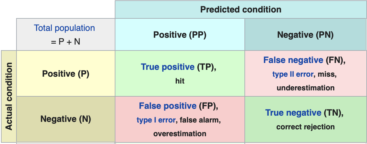
Where:

True positive (TP): a test result that correctly indicates the presence of a condition or characteristic
True negative (TN): a test result that correctly indicates the absence of a condition or characteristic
False positive (FP or Type I Error): a test result which wrongly indicates that a particular condition or attribute is present
False negative (FN or Type II Error): a test result which wrongly indicates that a particular condition or attribute is absent

Precision

Precision measures how the model is accurate for the positive predictions:

\[Precision=\frac{TP}{TP+FP}\]

Recall (or Sensitivity, Hit Rate or True Positive Rate)

Recall measures the percentage of the positive population that was detected positive:

\[Recall=\frac{TP}{TP+FN}=\frac{TP}{P}\]

False Positive Rate

False Positive Rate measures the percentage of the negative population that was detected positive:

\[Recall=\frac{FP}{FP+TN}=\frac{TP}{P}\]

Specificity (or Selectivity or True Negative Rate)

Specificity measures the percentage of the negative population that was detected negative:

\[Specificity=\frac{TN}{TN+FP}=\frac{TN}{N}\]

F1-Score

\(F_1\)-Score is an harmonic mean of precision and recall. For two number \(X_1\) and \(X_2\), the harmonic mean is:

\[H(X_1, X_2)=2 \times \frac{X_1 X_2}{X_1 + X_2}\]

So the \(F_1\)-Score is:

\[F_1=2 \times \frac{Precision \times Recall}{Precision + Recall}\]

Accuracy

Accuracy which is a natural metric is just the percentage of well predict samples:

\[Accuracy = \frac{TP + TN}{TP + TN + FP + FN} = \frac{TP + TN}{n}\]

Where:

\(n\) is the total number of samples.

ROC Curve

ROC (for Receiver operating characteristic) Curve is a curve created where each point corresponds to the results obtained for a given threshold. It plots, for every thresholds, the True Positive Rate against the False Positive Rate:

For a threshold of 0, the TPR would be 1 (every element of the positive population detected positive) and the FPR would also be 1 (every element of the negative population detected positive).

For a threshold of 1, the TPR would be 0 (every element of the positive population detected negative) and the FPR would also be 0 (no element of the negative population detected positive).

Other threshold are in between. A perfect classifier would have a TPR of 1 every element of the positive population detected positive) and a FPR of 0 (no element of the negative population detected positive).

AUC

AUC for Area Under Curve is the area under the ROC curve or its integral. When using normalized units, AUC is equal to the probability that a classifier will rank a randomly chosen positive instance higher than a randomly chosen negative one.

AUC is related to the Mann–Whitney U and to the Gini coefficient (not the Gini impurity).

See the paragraph dedicated to AUC on the Wikipedia page for ROC Curve.

Resources

For all of the classification metrics see:

Wikipedia page on ROC Curve (with references to other classification metrics).

Unsupervised Metrics

Most of unsupervised metrics (without labels) are based on the variance intra clusters and the variance inter cluster.

Silhouette coefficient

Silhouette coefficient is a clustering metric defined for a single cluster as:

\[s=\frac{b-a}{\max(a,b)}\]

Where:

a is the mean distance between a sample and all other points in the same cluster (or class),
b is the mean distance between a sample and all other points in the next nearest cluster.

For a set of cluster in is then:

\[s=\frac{1}{n_{clusters}}\sum_{i=1}^{n_{clusters}}\frac{b_i-a_i}{\max(a_i,b_i)}\]

If a cluster is very dense and far from its nearest neighbours then is silhouette coefficient will be high. On the contrary a sparse cluster not isolated from its neighbours will have a low silhouette coefficient.

Pros and Cons

Pros

The score is bounded between -1 for incorrect clustering and +1 for highly dense clustering. Scores around zero indicate overlapping clusters,
The score is higher when clusters are dense and well separated, which relates to a standard concept of a cluster.

Cons

The Silhouette Coefficient is generally higher for convex clusters than other concepts of clusters, such as density based clusters like those obtained through DBSCAN.

Calinski-Harabasz Index

Calinski-Harabasz Index is a clustering metric defined, for a dataset \(E\) as:

\[s=\frac{B}{W}\frac{n_E-k}{k-1}\]

Where \(B_k\) is the between group dispersion measure and \(W_k\) is the within-cluster dispersion measure defined by:

\(B=\sum_{q=1}^{k}\sum_{x \in C_q}(x-c_q)(x-c_q)^t\),
\(W=\sum_{q=1}^{k}n_q(c_q-c_E)(c_q-c_E)^t\).

With:

\(C_q\) the set of points in cluster \(q\),
\(c_q\) the center of cluster \(q\),
\(c_E\) the center of E (center of the dataset),
\(n_E\) the size of the dataset (number of data points),
\(n_q\) the number of data points in the cluster \(q\).

The Calinski-Harabasz index is thus the ratio of the sum of between-clusters dispersion (variance inter) and of within-cluster dispersion (variance intra) for all clusters (where dispersion is defined as the sum of distances squared): The \(\frac{n_E-k}{k-1}\) is a penalty on the number of cluster.

For Calinski-Harabasz Index, an higher score is better.

Pros and Cons

Pros

The score is higher when clusters are dense and well separated, which relates to a standard concept of a cluster,
The score is fast to compute.

Cons

The Calinski-Harabasz index is generally higher for convex clusters than other concepts of clusters, such as density based clusters like those obtained through DBSCAN.

Davies-Bouldin Index

Davies-Bouldin Index is a clustering metric defined, for a dataset \(E\) as:

\[DB=\frac{1}{k}\sum_{i=1}^k \max_{i \ne j}R_{ij}\]

Where:

\(R_{ij}=\frac{s_i + s_j}{d_{ij}}\),

With:

\(s_i\) the average distance between each point of cluster and the centroid of that cluster – also know as cluster diameter,
\(d_{ij}\) the distance between cluster centroids \(i\) and \(j\).

By taking, for each \(i\), the maximum score \(R_{ij}\) the Davies-Bouldin Index just looks at the score for cluster \(i\) compare to its closest neighbour (similar to Silhouette score). It will compare this distance to the sum of the average distance in cluster \(i\) and in cluster \(j\).

Zero is the lowest possible score. Values closer to zero indicate a better partition.

Pros and Cons

Pros

The computation of Davies-Bouldin is simpler than that of Silhouette scores,
The index is solely based on quantities and features inherent to the dataset as its computation only uses point-wise distances.

Cons

The Davies-Boulding index is generally higher for convex clusters than other concepts of clusters, such as density based clusters like those obtained from DBSCAN,
The usage of centroid distance limits the distance metric to Euclidean space.

Resources

See:

Scikit-Learn page on Unsupervised metrics.

Other metrics

See:

CS230 section 8 for other metrics.