Revision

Machine Learning

Definition

Gaussian discriminant analysis (GDA) is a binary classification model which tries to estimate the distribution of the input \(X\) given the output class \(Y\), ie \(p(X \vert Y)\).

The model learns the conditional distribution of \(X\) given \(Y\) during training and for inference it will compare the distribution of the true \(X\) to the expected distribution of the difference class \(Y\) (ie class 0 and 1 - \(p(X \vert 0)\) and \(p(X \vert 1)\)). The class attributed to \(X\) will be the one that match the best the distribution of \(X\). The tool used here in the Baye’s theorem.

In Gaussian discriminant analysis (GDA) the distributions of the inputs \(X\) given \(Y\) follow a normal distribution. The goal of the GDA is to find the parameters of the distribution for every output class.

Baye’s theorem

The Baye’s theorem is:

\[p(y \vert x) = \frac{p(x \vert y)p(y)}{p(x)}\]

It is just a derivation of this:

\[p(y \vert x) = p(x \cap y) = p(x \vert y)p(y)\]

Another formulation is:

\[posterior = \frac{prior \times likelihood}{evidence}\]

When looking for the \(y\) that maximises this probability we can get rid of the denominator as it does not depend on \(y\):

\[\begin{eqnarray} \arg \max_{y} p(y \vert x) &&= \arg \max_{y} \frac{p(x \vert y)p(y)}{p(x)} \\ &&= \arg \max_{y} p(x \vert y)p(y) \end{eqnarray}\]

It is the same for the GDA, we won’t have to compute the distribution of \(X\).

Formula

Multivariate gaussian

For a dimension \(d\) greater than 1, the normal distribution is:

\[p(x;\mu,\Sigma) = \frac{1}{(2\pi)^{d/2}\vert \Sigma \vert^{d/2}} \exp \left(-\frac{1}{2}\ (x-\mu)^T \Sigma^{-1} (x-\mu)\right)\]

Where:

The mean vector is \(\mu\),
The Variance-Covariance matrix is \(\Sigma\), \(\Sigma \in \mathbb{R}^{d\times d}\),
\(\vert \Sigma \vert\) is the determinant of the Variance-Covariance matrix \(\Sigma\),
The distribution is \(p(x;\mu,\Sigma) \sim \mathcal{N}(\mu, \Sigma)\).

Model

The Gaussian discriminant analysis is:

\[\begin{eqnarray} Y &&\sim \mathcal{B}(\phi) \\ X \vert Y=0 &&\sim \mathcal{N}(\mu_0, \Sigma) \\ X \vert Y=1 &&\sim \mathcal{N}(\mu_1, \Sigma) \end{eqnarray}\]

Writing the distribution we get:

\[\begin{eqnarray} p(Y) &&= \phi^Y (1-\phi)^{1-Y} \\ p(X \vert Y=0) &&= \frac{1}{(2\pi)^{d/2}\vert \Sigma \vert^{d/2}} \exp \left(-\frac{1}{2}\ (x-\mu_0)^T \Sigma^{-1} (x-\mu_0)\right) \\ p(X \vert Y=1) &&= \frac{1}{(2\pi)^{d/2}\vert \Sigma \vert^{d/2}} \exp \left(-\frac{1}{2}\ (x-\mu_1)^T \Sigma^{-1} (x-\mu_1)\right) \end{eqnarray}\]

Where:

The probability \(p(Y)\) (ie \(p(Y=0)\) and \(p(Y=1)\)) is call the prior: it is the probability of being of one class without any information on the individu (it is the proportion of each class in the population),
\(p(x \vert y)\) represents the probability distribution of each class,
The probabilities \(p(Y=0 \vert X)\) and \(P(Y=1 \vert X)\) are called the posterior as they represent the probability for \(X\) of being of one class given its caracteristics.

Assumption on the variance-covariance matrix

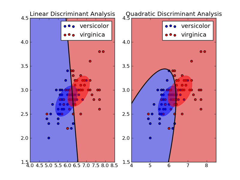
Here we make the assumption that the variance of \(X\) is not conditional to the class. This model, part of the GDA familly is called Linear Discriminant Analysis. Without this assumption the model is called Quadratic Discriminant Analysis.

To summarize:

If \(\Sigma_0 = \Sigma_1\): Linear Discriminant Analysis as the frontier is linear,
If \(\Sigma_0 \neq \Sigma_1\): Quadratic Discriminant Analysis as the frontier is quadratic.

Calibration using MLE

The model is calibrated using the maximum likelihood estimation.

We want to maximise the joint probability of having \(X\) and \(Y\).

By definition \(p(X \cap Y) = p(X, Y) = p(X \vert Y)p(Y)\) and we get \(L\) the MLE loss:

\[\begin{eqnarray} L(\phi,\mu_{0},\mu_{1},\Sigma) && = \prod_{j=1}^{n_{pop}} p\left(X^{(j)}, Y^{(j)}; \phi, \mu_{0}, \mu_{1}, \Sigma\right) \\ && = \prod_{j=1}^{n_{pop}} p\left(X^{(j)} | Y^{(j)}; \mu_{0}, \mu_{1}, \Sigma\right) p(Y^{(j)}; \phi) \\ && = \prod_{j=1}^{n}\phi^{Y^{(j)}}(1-\phi)^{1-Y^{(j)}} \frac{1}{(2\pi)^{d/2}|\Sigma|^{1/2}}\exp \left(-\frac{1}{2}(X^{(j)}-\mu_{Y^{(j)}})^{T}\Sigma^{-1}(X^{(j)}-\mu_{Y^{(j)}})\right) \end{eqnarray}\]

Where:

\(\mu_{y^{(j)}}\) is \(\mu_0\) if \(Y==0\) and \(\mu_1\) if \(Y=1\).

Applying the log (monotone strictly increasing function), we obtain:

\[\begin{eqnarray} l(\phi,\mu_{0},\mu_{1},\Sigma) &&= \log L(\phi,\mu_{0},\mu_{1},\Sigma) \\ &&= \sum_{j=1}^{n_{pop}} \left(Y^{(j)} \log \phi + (1-Y^{(j)}) \log(1-\phi) - \frac{1}{2} \log(2\pi) -\frac{1}{2} \log |\Sigma| - \frac{1}{2} (X^{(j)} - \mu_{Y^{(j)}})^{T} \Sigma^{-1} (X^{(j)}-\mu_{Y^{(j)}})\right) \end{eqnarray}\]

We can analytically maximize this function with respect to the different parameters by setting their derivatives to 0.

Resolution for \(\phi\)

\[\begin{eqnarray} \frac{d l}{d \phi} && = \frac{d}{d \phi} \sum_{j=1}^{n_{pop}}\left(Y^{(j)}\log\phi+(1-Y^{(j)})\log(1-\phi)\right) \\ && = \sum_{j=1}^{n_{pop}}\frac{d(Y^{(j)}\log\phi)}{d \phi} + \frac{d\left((1-Y^{(j)})\log(1-\phi)\right)}{d \phi} \\ && = \frac{\sum_{j=1}^{n_{pop}}Y^{(j)}}{\phi} - \frac{\sum_{j=1}^{n_{pop}}(1-Y^{(j)})}{1-\phi} \\\\ \text{Setting derivative to 0 } && \Rightarrow \frac{\sum_{j=1}^{n_{pop}}Y^{(j)}}{\phi} - \frac{\sum_{j=1}^{n_{pop}}(1-Y^{(j)})}{1-\phi} = 0 \\ && \Rightarrow \ \frac{\sum_{j=1}^{n_{pop}}Y^{(j)}}{\phi} = \frac{\sum_{j=1}^{n_{pop}}(1-Y^{(j)})}{1-\phi} \\ && \Rightarrow \ \sum_{j=1}^{n_{pop}}Y^{(j)}-\phi\sum_{j=1}^{n_{pop}}Y^{(j)} = n_{pop} \phi - \phi \sum_{j=1}^{n_{pop}}Y^{(j)} \\ && \Rightarrow \ \phi = \frac{\sum_{j=1}^{n_{pop}} Y^{(j)}} {n_{pop}} \\ && \Rightarrow \ \phi = \frac{\sum_{j=1}^{n_{pop}} [Y^{(j)} = 1]} {n_{pop}} \end{eqnarray}\]

\(\phi\) is simply the proportion of individuals of class 1 in the population.

Resolution for \(\mu_0\) and \(\mu_1\)

\[\begin{eqnarray} \frac{d l}{d \mu_{0}} &&= \frac{d}{d \mu_{0}}\sum_{j=1}^{n_{pop}} - \frac{1}{2}(X^{(j)}-\mu_{Y^{(j)}})^{T}\Sigma^{-1}(X^{(j)}-\mu_{Y^{(j)}}) \\ &&= -\frac{1}{2}\sum_{j=1}^{n_{pop}} \left(\frac{d(X^{(j)}-\mu_{Y^{(j)}})^{T}\Sigma^{-1}(X^{(j)}-\mu_{Y^{(j)}})}{d (X^{(j)}-\mu_{Y^{(j)}})}\right)\frac{d(X^{(j)}-\mu_{Y^{(j)}})}{d \mu_{0}} \\ &&= \Sigma^{-1}\sum_{j=1}^{n_{pop}} (X^{(j)}-\mu_{0})[Y^{(j)}=0] \\\\ \text{Setting derivative to 0 } && \Rightarrow \ \sum_{j=1}^{n_{pop}} (X^{(j)}-\mu_{0})[Y^{(j)}=0] = 0 \\ && \Rightarrow \ \sum_{j=1}^{n_{pop}} X^{(j)}[Y^{(j)}=0] = \mu_{0}\sum_{j=1}^{n_{pop}} [Y^{(j)}=0] \\ && \Rightarrow \ \mu_{0} = \frac{\sum_{j=1}^{n_{pop}}X^{(j)}[Y^{(j)}=0]}{\sum_{j=1}^{n_{pop}} [Y^{(j)}=0]} \end{eqnarray}\]

Equivalently for \(\mu_1\) we get:

\[\mu_{1} = \frac{\sum_{j=1}^{n_{pop}}X^{(j)} [Y^{(j)} = 1]} {\sum_{j=1}^{n_{pop}}[Y^{(j)} = 1]}\]

\(\mu_0\) and \(\mu_1\) are just the average of the individuals caracteristics of each class.

Resolution for \(\Sigma\)

With the assumption that \(\Sigma_0 = \Sigma_1\) (LDA) we get:

\[\begin{eqnarray} \frac{d l}{d \Sigma} && = \frac{d}{d \Sigma} \left[\sum_{j=1}^{n_{pop}}\frac{1}{2}\log|\Sigma^{-1}|-\frac{1}{2}(X^{(j)}-\mu_{Y^{(j)}})^{T}\Sigma^{-1}(X^{(j)}-\mu_{Y^{(j)}}) \right]\\ && = \frac{d}{d \Sigma}\sum_{j=1}^{n_{pop}} \left[\frac{1}{2}\log|\Sigma^{-1}|\right] - \frac{d}{d \Sigma}\sum_{j=1}^{n_{pop}} \left[\frac{1}{2}tr\left((X^{(j)}-\mu_{Y^{(j)}})(X^{(j)}-\mu_{Y^{(j)}})^{T}\Sigma^{-1}\right)\right] \\ && = \left[\frac{n}{2}\frac{1}{\Sigma^{-1}} \frac{d \Sigma^{-1}}{d \Sigma}\right] - \left[\frac{1}{2} \frac{d \Sigma^{-1}}{d \Sigma} \sum_{j=1}^{n_{pop}}(X^{(j)}-\mu_{Y^{(j)}})(X^{(j)}-\mu_{Y^{(j)}})^{T}\right] \\\\ \text{Setting derivative to 0 } && \Rightarrow \ \frac{n}{2}\frac{1}{\Sigma^{-1}} \frac{d \Sigma^{-1}}{d \Sigma} - \frac{1}{2} \frac{d \Sigma^{-1}}{d \Sigma} \sum_{j=1}^{n_{pop}}(X^{(j)}-\mu_{Y^{(j)}})(X^{(j)}-\mu_{Y^{(j)}})^{T} = 0\\ && \Rightarrow \ \frac{n}{2} \Sigma \frac{d \Sigma^{-1}}{d \Sigma} = \frac{1}{2} \frac{d \Sigma^{-1}}{d \Sigma} \sum_{j=1}^{n_{pop}}(X^{(j)} - \mu_{Y^{(j)}})(X^{(j)} - \mu_{Y^{(j)}})^{T} \\ && \Rightarrow \ n \Sigma = \sum_{j=1}^{n_{pop}}(X^{(j)} - \mu_{Y^{(j)}})(X^{(j)} - \mu_{Y^{(j)}})^{T} \\ && \Rightarrow \ \Sigma = \frac{1}{n} \sum_{j=1}^{n_{pop}}(X^{(j)} - \mu_{Y^{(j)}})(X^{(j)} - \mu_{Y^{(j)}})^{T} \end{eqnarray}\]

Without the assumption \(\Sigma_0 = \Sigma_1\) (QDA) we get (using the same steps):

\[\Sigma_0=\frac{1}{(n_{pop})^0}\sum_{j=1}^{(n_{pop})^0}(X^{(j)}-\mu_0)(X^{(j)}-\mu_0)^{T}\mathbb 1\!\!1_{Y^{(j)} = 0}\] \[\Sigma_1=\frac{1}{(n_{pop})^1}\sum_{j=1}^{(n_{pop})^1}(X^{(j)}-\mu_1)(X^{(j)}-\mu_1)^{T}\mathbb 1\!\!1_{Y^{(j)} = 1}\]

Inference

Now that all the parameters are calibrated, for inference we will just get the the class \(Y\) with maximum \(p(Y \vert X)\). Using Bayes theorem and the properties of max we get:

\[\begin{eqnarray} Y &&= \max_Y p(Y \vert X) &&= \max_Y \frac{p(X \vert Y)p(Y)}{p(X)} &&= \max_Y p(X \vert Y)p(Y) \end{eqnarray}\]

Using the parameters we can compute \(p(X \vert Y)\) and \(p(Y)\) for \(Y=0\) and \(Y=1\).

Link with logistic regression

If we view the quantity \(p(Y = 1 \vert X; \phi, \mu_0, \mu_1, \Sigma)\) as a function of \(X\), we’ll find that it can be expressed in the form:

\[p(Y = 1 \vert X; \phi, \mu_0, \mu_1, \Sigma) = \frac{1}{1+\exp(-\theta^T X)}\]

Where \(\theta\) depends on \(\phi, \mu_0, \mu_1, \Sigma\).

Hence it is the same form as the logistic regression.

The only difference is that GDA assumes that the distribution of \(p(X \vert Y)\) is gaussian but the logistic regression does not make this assumption.

Frontiers of LDA and QDA

LDA

The frontier for the LDA is:

\[2(\Sigma^{-1}(\mu_1-\mu_0))^T X + (\mu_1 - \mu_0)^T\Sigma^{-1}(\mu_1 - \mu_0) + 2\log(\frac{1-\phi}{\phi}) = 0\]

It can be easily derived starting from \(p(Y=0 \vert X) = p(Y=1 \vert X)\) and expending the distribution.

The form of the equation is \(aX + b = 0\), hence it is linear.

QDA

The frontier for the QDA is:

\[X^T (\Sigma_0-\Sigma_1)^{-1} X + 2 (\mu_0^T\Sigma_0^{-1} - \mu_1^T\Sigma_1^{-1})^T X + 2 \log (\frac{1-\phi}{\phi}) + \log (\frac{|\Sigma_0|}{|\Sigma_1|}) + (\mu_1^T\Sigma_1^{-1}\mu_1 - \mu_0^T\Sigma_0^{-1}\mu_0) = 0\]

It can be easily derived starting from \(p(Y=0 \vert X) = p(Y=1 \vert X)\) and expending the distribution.

The form of the equation is \(aX^2 + bX + C = 0\), hence it is quadratic.

Resources

See:

CS229.