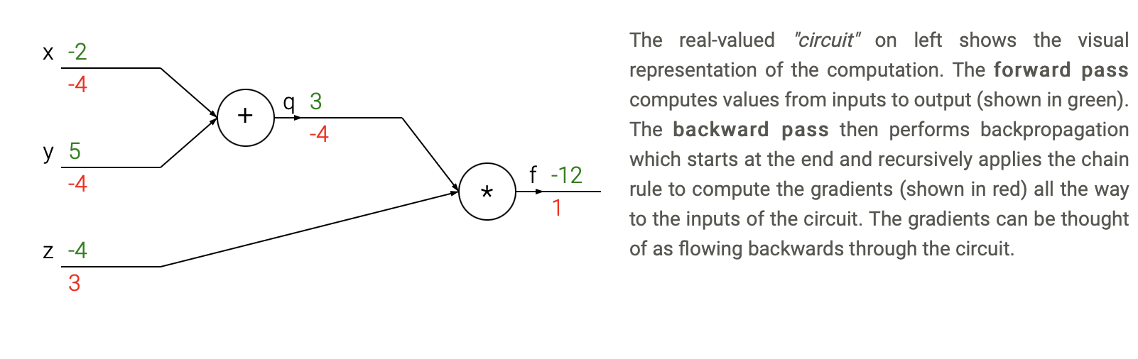
Backpropagation is an algorithm that computes the gradient of the loss function with respect to the weights of the neural network.
It is a way of performing gradient descent with respect to the given loss on each weight (each parameter) of the network.
Chain rule is the way of computing gradient of complex function by squashing the function in simple part and compound their gradient.
If:
\[h(x) = f(g(x))\]then:
\[h'(x)=f'(g(x))g'(x)\]Equivalently if:
\[h=f\circ g\]then:
\[h'=(f \circ g)' = (f' \circ g)\cdot g'\]Also equivalently if:
then:
\[\frac{dz}{dx} = \frac{dz}{dy} \cdot \frac{dy}{dx}\]The generalisation to \(n\) composed functions \(f_n \circ f_{n-1} \circ \cdots \circ f_2 \circ f_1\) is:
\[\frac{df_{n}}{dx} = \frac{df_{n}}{df_{n-1}} \frac{df_{n-1}}{df_{n-2}} \cdots \frac{df_{1}}{dx}\]See: Wikipedia page on Chaine rule.
Let denote our loss by \(C\). The gradient with respect to the input x is:
Where:
It can also be rewrite:
\[\nabla_{x}C = (W^{1})^{T} \cdot (f^{1})' \ldots \circ (W^{L-1})^{T} \cdot (f^{L-1})' \circ (W^{L})^{T} \cdot (f^{L})' \circ \nabla_{x^{L+1}}C\]Where \(\nabla_{x}\) is the gradient of \(C\) wrt \(x\).
Let’s define \(\delta\) such that:
\[\delta^l := (f^{l})' \circ (W^{l+1})^{T} \cdots \circ (W^{L-1})^{T}\cdot (f^{L-1})' \circ (W^{L})^{T} \cdot (f^{L})' \circ \nabla_{x^{L+1}}C\]\(\delta^l\) is the derivative wrt to \(x^l\).
What we are looking for is the gradient of the weights. These are the parameters that we are going to tune (getting the gradient wrt to the input won’t be useful to train the network - but it may be useful to check which part of the input lead to a wrong prediction).
The gradient wrt to \(W^l\) is:
\[\begin{eqnarray} \nabla_{W^{l}} C &&= \frac {dC}{dx^{L+1}} \cdot \frac {df^{L}(b^L + W^L x^L)}{d(b^L + W^L x^L)} \circ {\frac {d(b^L + W^L x^L)}{dx^L}} \ldots \frac {df^l (b^l + W^l x^l)}{d(b^l + W^l x^l)} \circ \frac {d(b^l + W^l x^l)} {dW^l} \\ &&= \frac{df^l}{dW^l} (f^{l})' \circ (W^{l+1})^{T} \cdots \circ (W^{L-1})^{T}\cdot (f^{L-1})' \circ (W^{L})^{T} \cdot (f^{L})' \circ \nabla_{x^{L+1}}C\\ &&= \frac{d(b^l + W^l x^l)}{dW^l} \delta^l\\ &&= \delta^l (x^l)^T \end{eqnarray}\]The gradients wrt to every parameters can be computed sequentially using the fact that:
\[\delta^{l-1}:=(f^{l-1})'\circ (W^{l})^{T}\cdot \delta ^{l}\]Training of a neural network is done through backpropagation which is equivalent to a Gradient Descent.
Generally in a neural network, the gradient descent is stochastic which means that only a sub sample of the training dataset is used at each iteration to compute the gradient.
Apart the classical Stochastic Gradient Descent method, other more complex and stable Gradient Descent methods have been created to improve stability and speed of the calibration of a neural network.
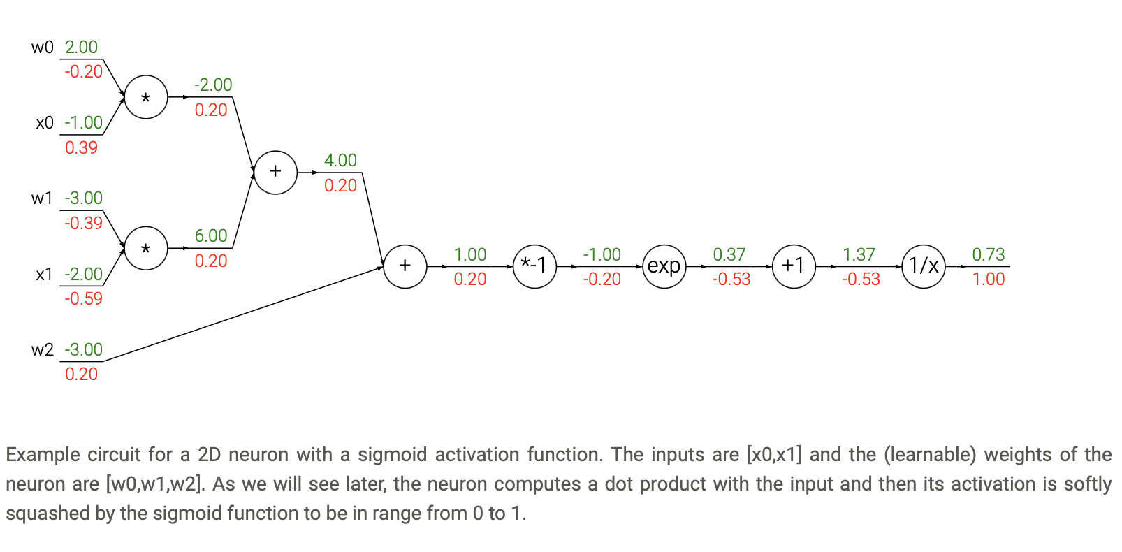
Images and texts are taken from CS231n.
See:
For a parameter \(W^{l}\) we saw that the gradient is:
\[\nabla_{W^{l}} C(X, Y) = \delta^l (x^l)^T\]Hence the gradient descent update rule is:
\[(W^{l})^{i+1} = (W^{l})^i - \alpha \nabla_{W^{l}} C(X, Y) = (W^{l})^i - \alpha \delta^l (x^l)^T\]Where:
The simplified form is:
\[W = W - \alpha \nabla_W C(X, Y)\]Or more simplified:
\[W = W - \alpha \nabla_W\]Stochastic Gradient Descent is equivalent to Gradient Descend but taken only on a batch \(B\) ie a sub sample of the dataset. Using a sub sample of data allows to compute more quicky the loss function and avoid to wait a long time before getting an update.
\[\nabla_{W^{l}} C(X_B, Y_B) = \delta^l (x_B^l)^T\]Hence the gradient descent update rule is:
\[(W^{l})^{i+1} = (W^{l})^i - \alpha \nabla_{W^{l}} C(X_B, Y_B) = (W^{l})^i - \alpha \delta^l (x_B^l)^T\]The simplified form is:
\[W = W - \alpha \nabla_W C(X_B, Y_B)\]And more simplified by not expressing the loss and the dataset we obtain the same representation than for normal gradient descent:
\[W = W - \alpha \nabla_W\]For the next methods, we will use simplified notations.
However keep in mind that:
Their exist two families of SGD upgrades:
The momentum methods introduce a variable \(v\) for velocity and the gradient will update the velocity of updates not directly the parameter.
When using gradient descent a tradeoff exists between the time taken to converge and the precision of the convergence.
The parameter \(\alpha\) is used to modify the step size. A large \(\alpha\) will induce large steps and a small \(\alpha\) small steps. In general we want to make large steps at the begining of the training and smaller steps at the end. The \(\alpha\) parameter can be decayed during the training:
The Adaptive learning rate methods include adaptation of the learning rate direclty based on the derivatives values.
The update rule using the momentum method is:
\[\begin{cases} v = \mu v - \alpha \nabla_W \\ W = W + v \end{cases}\]Where:
The method is called momentum as the gradient keep a trace of the precedent gradient direction and hence follows the momentum.
Nesterov Momentum is similar to Momentum. The update rule using the Nesterov momentum method is:
\[\begin{cases} W_{ahead} = W + \mu v \\ v = \mu v - \alpha \nabla_{W_{ahead}} \\ W = W + v \end{cases}\]Nesterov Momentum still uses the momentum ie keeps trace of the precedent gradient direction but it will compute the update to the variable \(v\) with respect to \(W_{ahead}\) ie the \(W\) variable where another gradient step has been applied.
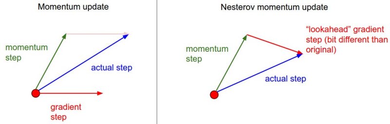
Instead of evaluating gradient at the current position (red circle), we know that our momentum is about to carry us to the tip of the green arrow. With Nesterov momentum we therefore instead evaluate the gradient at this “looked-ahead” position.
From CS231n course.
Adagrad is an adaptive learning rate method. The update rule using the Adagrad method is:
\[\begin{cases} c = c + \nabla^2_W \\ W = W - \alpha \frac{\nabla_W}{\sqrt{c} + \varepsilon} \end{cases}\]Where:
Weights that receive high gradients will have their effective learning rate reduced, while weights that receive small or infrequent updates will have their effective learning rate increased
RMSprop is an adaptive learning rate method. The update rule using the RMSprop method is:
\[\begin{cases} c = \gamma c + (1 - \gamma) \nabla^2_W \\ W = W - \alpha \frac{\nabla_W}{\sqrt{c} + \varepsilon} \end{cases}\]RMSprop is similar to Adagrad but the variable \(c\) acts like a weigted sum of the last squared gradient.
ADAM is an adaptive learning rate and momentum method. The update rule using the ADAM method is:
\[\begin{cases} m = \beta_1 m + (1 - \beta_1) \nabla_W \\ v = \beta_2 v + (1 - \beta_2) \nabla^2_W \\ W = W - \alpha \frac{m}{\sqrt{v} + \varepsilon} \end{cases}\]Is is very similar to RMSprop but with momentum.
Here are some animations that may help the intuitions about the learning process dynamics:
Contours of a loss surface and time evolution of different optimization algorithms. Notice the “overshooting” behavior of momentum-based methods, which make the optimization look like a ball rolling down the hill.
A visualization of a saddle point in the optimization landscape, where the curvature along different dimension has different signs (one dimension curves up and another down). Notice that SGD has a very hard time breaking symmetry and gets stuck on the top. Conversely, algorithms such as RMSprop will see very low gradients in the saddle direction. Due to the denominator term in the RMSprop update, this will increase the effective learning rate along this direction, helping RMSProp proceed.
Images credit: Alec Radford.
Second order methods based on Newton’s method automatically adapt the step size given the second derivative of the loss. They used a second order approximation of a the Taylor series of a function \(f\).
However this approximation uses the Hessian matrix of the function and the computing (and inverting) the Hessian matrix of a neural network is very costly in time and memory.
Hence Newton’s method is not use to calibrate neural networks.
See: