Revision

Back to Deep Reinforcement Learning

Introduction

Deep Reinforcement Learning is the application of (deep) neural network for reinforcement learning.

Motivation

The classical approaches deal with finite Markov Decision Process with a finite number of states and actions. However in real applications, the number of states and actions can be infinite if the states and actions are continuous values.

They use tables to store state value function and action value function (the \(Q\)-table for example). The term function is used in these method to refer to state and action value functions but these functions must be seen as mapping or tables. In continuous environment using mapping or tables is no longer possible.

Deep Reinforcement methods can deal continuous (inifinite) states space and (for some) continuous action space.

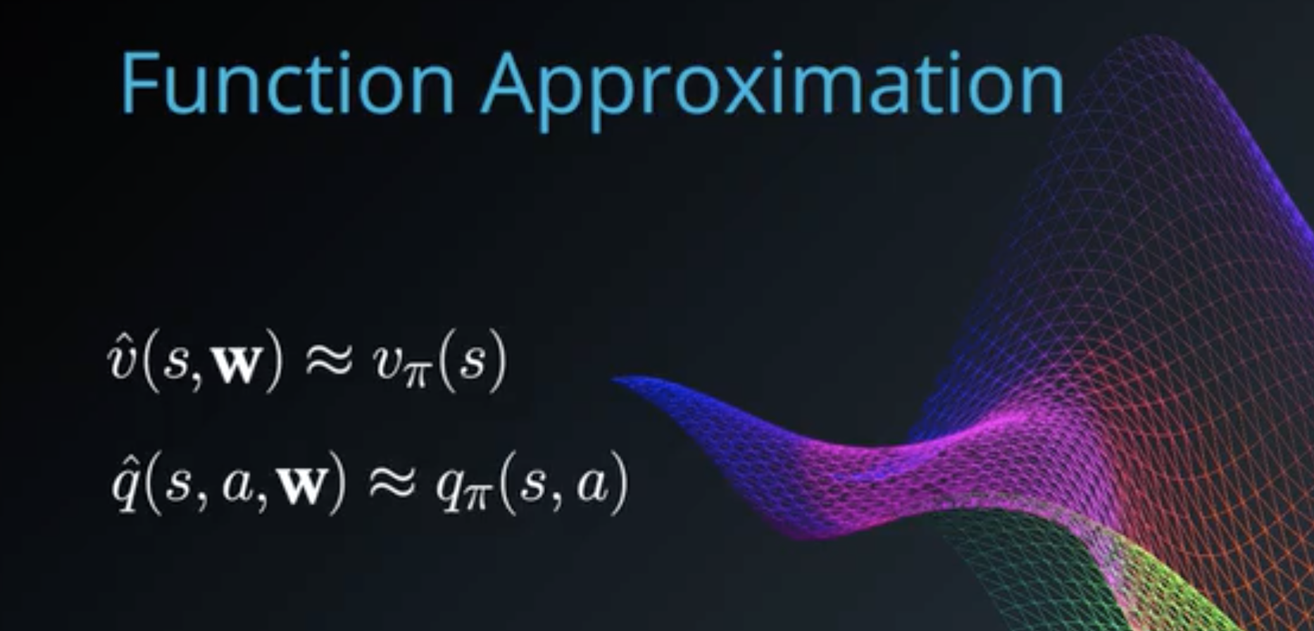
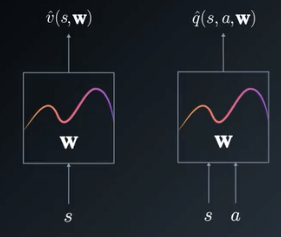
\(v_\pi\) and \(q_\pi\) are now true unknown continuous functions that we need to approximate. We thus seek \(\hat{v}\) and \(\hat{q}\) that will approximate \(v_\pi\) and \(q_\pi\).

Typically \(\hat{v}\) and \(\hat{q}\) will be parametrized by weights \(w\) and will be neural networks:

Also in Deep Reinforcement Learning the steps of estimating the value functions (state or action or both) and then updating the policy using the \(\varepsilon\)-greedy method is done at the same time. The value functions are updated and the policy is also updated at the same time.

Real example of continuous state and action spaces

A car moves in a continuous environment with continuous actions:

• The position of the car is continous, its speed is continuous and the angle of the car is continuous,
• The agent can choose to accelerate or decelerate but it can also decides how much to accelerate or decelerate,
• It can decide to go left or right but can also decide the exact angle.

Notation

Let’s introduce some notations:

• \(\hat{v}(s, w)\) represents the approximation of the state value function, \(s\) being a state and \(w\) the parameters of the approximation function,
• \(\hat{a}(s, a, w)\) represents the approximation of the action value function, \(s\) being a state, \(a\) being an action and \(w\) the parameters of the approximation function,
• \(x(s)=(x_1(s), x_2(s), \ldots, x_n(s))\) represents the \(n\) features of state \(s\): position, speed, angle, quantities of anything, etc. (or image of the visible environment),
• \(x(s, a)=(x_1(s, a), x_2(s, a), \ldots, x_n(s, a))\) represents the \(n\) features of state \(s\) and action \(a\): position, speed, angle, quantities of anything, etc. (or image of the visible environment).