Revision

Back to Probability distribution

Distributions

Continuous Uniform

Let \(\mathcal{U}(a,b)\) be an continuous uniform distribution on \([a, b]\). A random sampling following \(\mathcal{U}(a,b)\) outputs any value between \(a\) and \(b\) with an equal probability. The continuous uniform distribution is a continuous distribution with support \([a, b]\).

pdf and cdf

Mathematically, its probability density function is:

\[f(x;a,b)=\begin{cases} \frac{1}{b-a} && \text{ if } a \leq x \leq b\\ 0 && \text{ otherwise} \end{cases}\]

And its cumulative density function is:

\[F(x;a,b)=\begin{cases} 0 && \text{ if } x \lt a\\ \frac{x-a}{b-a} && \text{ if } a \leq x \leq b\\ 0 && \text{ if } x \gt b\\ \end{cases}\]

Moments

For \(U \sim \mathcal{U}(a,b)\):

\(\mathbb{E}(U)=\frac{a+b}{2}\),
\(Var(U)=\frac{(b-a)^2}{12}\) (see this StackExchange page for a proof).

Complementary infos

The cumulative function \(F\) of a probability distribution applied to a random variable \(X\) that follows this distribution is a random variable that follows the uniform distribution: \(F_X(X) \sim \mathcal{U}(0,1)\)

Proof

Let X be a random variable with cdf \(F_X(X)\) and let \(U=F_X(X)\). By definition of the cdf, \(U \in [0,1]\).

Note that the cdf is a continuous increasing function.

U is a random variable as U is a transformation of X, X being a random variable.

Let \(F_U(x)\) be the cdf of U:

\[F_U(x)=P(U \leq x)=P(F_X(X) \leq x)=P(X \leq F_X^{-1}(x))=F_X(F_X^{-1}(x))=x\]

Use of the definition of the cdf
Use of \(U=F_X(X)\)
Use the fact that \(F_X^{-1}(F_X(X))=X\) and that \(F_X(X)\) is a continuous increasing function
Use again the definition of the cdf
Use \(F_X^{-1}(F_X(x))=x\)

So \(F_U(x)=x\) with U taking value in [0, 1], so \(F_U(x)\) is equivalent to a cdf of a uniform variable on [0, 1] so \(U \sim \mathcal{U}(0,1)\).

Reference

See Wikipedia webpage of Continuous Uniform distribution.

Discrete uniform

Let \(\mathcal{U}(A,B)\) be an uniform distribution on \([A, B]\). A random sampling following \(\mathcal{U}(A,B)\) outputs any integer value between \(A\) and \(B\) with an equal probability. The discrete uniform distribution is a continuous distribution with support \(k \in \{A, \ldots, B\}\).

pdf and cdf

Mathematically, its probability mass function is:

\[f(k;A,B)=\begin{cases} \frac{1}{B - A +1} && \text{ if } A \leq k \leq B\\ 0 && \text{ otherwise} \end{cases}\]

And its cumulative density function is:

\[F(k;A,B)=\begin{cases} 0 && \text{ if } k \lt A\\ \frac{\lfloor k \rfloor - A + 1}{B - A + 1} && \text{ if } a \leq k \leq b\\ 0 && \text{ if } k \gt b\\ \end{cases}\]

Moments

For \(U \sim \mathcal{U}(A,B)\):

\(\mathbb{E}(U)=\frac{A+B}{2}\),
\(Var(U)=\frac{(B - A + 1)^2 - 1}{12}\).

Reference

See Wikipedia webpage of Discrete Uniform distribution.

Reciprocal or log-Uniform

The reciprocal distribution, or log-uniform distribution, is a continuous probability distribution characterised by its probability density function being proportional to the reciprocal (the inverse, \(1/x\)) of the variable. The reciprocal distribution is a continuous distribution with support \([a, b]\).

pdf and cdf

Mathematically, its probability density function is:

\[f(x;a,b)=\begin{cases} \frac{1}{x \left[\log_e b - \log_e a\right]} = \frac{1}{x \log_e \frac{b}{a}} && \text{ if } a \leq x \leq b \text{ and } a \gt 0\\ 0 && \text{ otherwise} \end{cases}\]

Where:

\(\log_e\) is the \(\log\) function to base \(\exp\).

And its cumulative density function is:

\[F(x;a,b)=\begin{cases} 0 && \text{ if } x \lt a\\ \frac{\log_e x - \log_e a}{\log_e b - \log_e a} = \frac{\log_e \frac{x}{a}}{\log_e \frac{b}{a}} && \text{ if } a \leq x \leq b \text{ and } a \gt 0\\ 0 && \text{ if } x \gt b\\ \end{cases}\]

Moments

For \(U \sim \mathcal{U}(a,b)\):

\(\mathbb{E}(R)=\frac{b - a}{\log \frac{b}{a}}\),
\(Var(R)=\frac{b^2 - a^2}{2 \log \frac{b}{a}} - \left(\frac{b - a}{\log \frac{b}{a}}\right)^2\).

Link with log-Uniform

The reciprocal distribution is equivalent to the distribution of \(\log(X) \sim \mathcal{U}(\log a, \log b)\). This relationship is true regardless of the base of the logarithmic or exponential function. If \(\log_{m}(X)\) is uniform distributed, then so is \(\log_{n}(X)\).

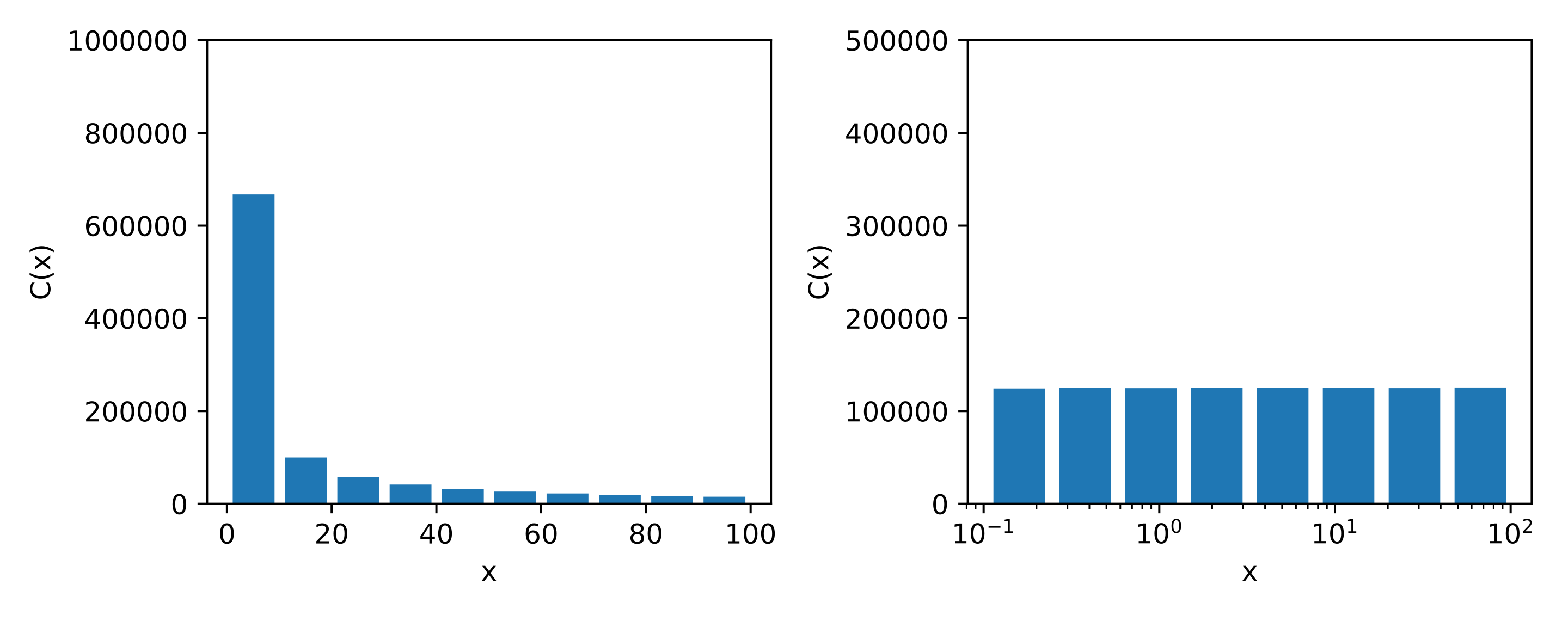
Histogram of the Reciprocal distribution \(\mathcal{R}(10^{-1}, 10^2)\) using normal basis and logarithmic basis.

Reference

See Wikipedia webpage of Reciprocal distribution.

Bernoulli

A Bernoulli random variable is a discrete random variable that takes the value 1 with probability \(p\) and value 0 with probability \(q=1-p\). The only parameter of \(\mathbb{B}(p)\) is p, the probability to obtain 1 and the support of \(\mathbb{B}(p)\) is \(\{0, 1\}\).

pdf and cdf

Its probability density function is:

\[P(Y=y)=\begin{cases} p && \text{ if } y=1\\ 1-p && \text{ if } y=0\\ 0 && \text{ otherwise}\ \end{cases}\]

Or equivalently:

\[P(Y=y)=p^y(1-p)^y \text{ for } y \in \{0, 1\}\]

(This reformulation is used in the construction of the logistic regression loss function).

The cumulative density function is not very useful, its value is \(q=1-p\) on the support.

Moments

For \(B \sim \mathcal{B}(p)\):

\(\mathbb{E}(B)=p\),
\(Var(B)=pq=p(1-p)\).

Reference

See Wikipedia webpage of Bernoulli distribution.

Binomial

A Binomial distribution is a discrete probability distribution with parameters n and p. It represents the number of success \(n\) Bernoulli trial where each experiment has a probability \(p\) of success (ie \(P[X=1]=p\)). It is written \(\mathbb{B}(n, p)\) and its support is discrete and is \(k \in {0, 1, ..., n}\).

pdf and cdf

Its probability density function is:

\[f(k,n,p)=P(X=k)={n \choose k}p^k q^{n-q}\]

Where k is a number of success and n the number of trials (and p and q the probability to obtain respectively 1 and 0 at each trial).

Its cdf is:

\[F(k,n,p)=P(X \leq k)=\sum_{i=0}^{\vert k \vert^{floored}}{n \choose i}p^i(1-p)^{n-i}\]

Moments

For \(B \sim \mathcal{B}(n,p)\):

\(\mathbb{E}(B)=np\),
\(Var(B)=npq=np(1-p)\).

Complementary infos

As the Central Limit Theorem says, the sum of iid variables converges to a gaussian distribution. As the binomial distribution is a sum of iid Bernoulli random variables then the Binomial distribution converges toward the gaussian distribution when n goes to infinity (see this stackexchange link).

Reference

See Wikipedia webpage of Binomial distribution.

Multinomial

A Multinomial distribution is a discrete distribution, generalisation of the Binomial distribution for trials with more than 2 possible outputs. Binomial distribution is the number of success of \(n\) Bernoulli trials and Multinomial distribution would be, for example, the number of counts for each side of a die rolled.

Its parameters are:

\(n\), the number of trials,
\(k\), the number of possible outcomes of each trial,
\(p_1, \ldots, p_k\) the probabilities of each outcome (\(\sum p_i = 1\)).

pdf and cdf

Its probability density function is:

\[f(x_1, \ldots, x_k,n,p) = \frac{\Gamma(\sum_i x_i + 1)}{\prod_i \Gamma(x_i + 1)} \prod_{i=1}p_i^{x_i}\]

Where \(x_i\) is the number of outcomes of class \(i\) (and \(\sum x_i = n\)).

Its cdf is:

\[\begin{eqnarray} F(x_1, \ldots, x_k,n,p) &&= P(X_1=x_1, \ldots, X_k=x_k) \\ &&=\frac{n!}{x_1! \cdots x_k!}p_1^{x_1} \times \cdots \times p_k^{x_k} \end{eqnarray}\]

Where \(x_i\) is the number of outcomes of class \(i\) (and \(\sum x_i = n\)).

Moments

For \(B \sim \mathcal{B}(n,p)\):

\(\mathbb{E}(X_i) = n p_i\),
\(Var(X_i) = n p_i (1 - p_i)\),
\(Cov(X_i, X_j) = - n p_i p_j \;\;\; i \neq j\).

Complementary infos

When \(x_i\) is large enough, we can apply CLT (as multinomial distribution is a some of random variable) and the multinomial distribution converges to the normal distribution:

\[\frac{x_i - n p_i}{\sqrt{n p_i(1 - p_i)}} \sim \mathcal{N}(0, 1)\]

and:

\[\sum_{i=1}^m \frac{(x_i - n p_i)^2}{\sqrt{n p_i(1 - p_i)}} \sim \chi_k^2\]

Reference

See :

Normal or Gaussian

Gaussian distribution is the most important distribution due to the Central Limit Theorem. Under certain conditions, the sum of iid random variables converges toward a gaussian distribution. In real world applications, most of the experiment follows normal distributions. It is a continuous distribution parametrized by its two first moment, its expected value \(\mu\) and its variance \(\sigma^2\). Its support is \(\mathbb{R}\).

pdf and cdf

The probability density function of the normal distribution is:

\[f(x;\mu,\sigma^2)=\frac{1}{\sigma \sqrt{2\pi}}e^{-\frac{1}{2}\left(\frac{x-\mu}{\sigma}\right)^2}\]

And its cumulative density function is in general expressed as the integral of the pdf:

\[F(x;\mu,\sigma^2)=\frac{1}{\sigma \sqrt{2\pi}}\int_{-\infty}^x e^{-\frac{1}{2}\left(\frac{t-\mu}{\sigma}\right)^2}dt\]

Moments

For \(N \sim \mathcal{N}(\mu,\sigma^2)\):

\(\mathbb{E}(N)=\mu\),
\(Var(N)=\sigma^2\),
Skewness=0,
Kurtosis=3.

Reference

See Wikipedia webpage of Normal distribution.

Chi-2

A Chi-2 distribution \(\chi^2(k)\) is a continuous distribution. It is parametrized by its degree of freedom \(k\).

A chi-2 with \(k\) degrees of freedom that can be defined as a sum of k variables \(Z \sim \mathcal{N}(0,1)\). Its support is \(\mathbb{R^+}\).

\[X(k) = \sum_{i=1}^{k} Z_i^2\]

Where:

\(Z_i \sim \mathcal{N}(0,1)\).

pdf and cdf

The probability density function of the chi-2 distribution is:

\[f(x;k)=\frac{1}{2^{k/2}\Gamma(k/2)}x^{k/2-1}e^{-x/2}\]

Where:

\(\Gamma(z)=\int_0^{+\infty}t^{z-1}e^{-t}dt\) is the gamma function (\(\Gamma(z+1)=z\Gamma(z)\)).

The cumulative density function of the chi-2 distribution is:

\[F(x;k)=\frac{\gamma \left(k/2, x/2 \right)}{\Gamma(k/2)}\]

Where:

\(\Gamma(z)\) is the gamma function,
\(\gamma(a,z)=\int_0^z t^{a-1}e^{-t}dt\) is the incomplete gamma function.

Moments

For \(X \sim \chi^2(k)\):

\(\mathbb{E}(X)=k\),
\(Var(X)=2k\).

Complementary infos

Using CLT, for \(k\) large enough, the Chi-2 distribution can be approximated by a normal distribution.

Reference

See Wikipedia webpage of Chi-2 distribution.

Student

A Student’s t-distribution \(\mathcal{T}(\nu)\) is a continuous density probability distribution widely used in statistical tests. It is parametrized by its degree of freedom \(\nu\) and its support is \(\mathbb{R}\).

It can be defined as a mean 0 and variance 1 normal variable divided by the square root of a chi-2 variable divided by it degree of freedom:

\[\mathcal{T}(\nu) = \frac{Z}{\sqrt{X/\nu}}\]

Where:

\(Z \sim \mathcal{N}(0,1)\),
\(X \sim \mathcal{X}(\nu)\) where \(\nu\) is its degree of freedom,
\(Z\) and \(X\) are independant.

pdf and cdf

Formulations of the pdf and cdf of the Student’s t-distribution are complex. See the Wikipedia webpage of the Student’s t-distribution to find them.

Moments

For \(T \sim \mathcal{T}(\nu)\):

\(\mathbb{E}(T)= \begin{cases} 0 \text{ if } \nu \gt 0 \\ \text{undefined otherwise} \end{cases}\),
\(Var(T)=\begin{cases} \frac{\nu}{\nu-2} \text{ if } \nu \gt 2 \\ \infty \text{ if } 1 \lt \nu \leq 2 \\ \text{undefined otherwise} \end{cases}\).

Reference

See Wikipedia webpage of the Student’s t-distribution.

Fisher

A Fisher distribution \(\mathcal{F}(d_1, d_2)\) is a continuous distribution. It is parametrized by two degree of freedom \(d_1\) and \(d_2\). These two degrees of freedom are the parameters of the two chi-2 distributions that defined the Fisher distribution, one at the numerator and the other at the denominator. The support of the Fisher distribution is \(\mathbb{R^+}\).

\[F(d_1, d_2)=\frac{X_1/d_1}{X_2/d_2}\]

Where:

\(X_1 \sim \mathcal{X}(d_1)\) where \(d_1\) is its degree of freedom,
\(X_2 \sim \mathcal{X}(d_2)\) where \(d_2\) is its degree of freedom.

pdf and cdf

Formulations of the pdf and cdf of the Fisher distribution are complex. See the Wikipedia webpage of the Fisher distribution to find them.

Reference

See Wikipedia webpage of the Fisher distribution.

Moments

For \(F \sim \mathcal{F}(d_1,d_2)\):

\(\mathbb{E}(F)= \frac{d_2}{d_2-2} \text{ if } d_2 \gt 2\),
\(Var(F)=\frac{2d_2^2\left(d_1+d_2-2\right)}{d_1\left(d_2-2\right)^2\left(d_2-4\right)} \text{ if } d_2 \gt 4\).

Poisson

A Poisson distribution is a discrete probability distribution \(\mathcal{P}(\lambda)\) that describes the number of events occuring in a time interval. Its support is \(\mathbb{N}\). A Poisson distribution has one parameter \(\lambda\) that represents the mean and variance of the distribution.

pdf and cdf

The probability density function of the Poisson distribution is:

\[f(k;\lambda)=\frac{e^{-\lambda}\lambda^k}{k!}\]

Where:

\(k\) is the number of occurrences.

The cumulative density function of the Poisson distribution is:

\[F(k;\lambda)=\frac{\Gamma\left(\vert k+1 \vert^{floored}, \lambda\right)}{\vert k \vert^{floored}!}= e^{-\lambda}\sum_{i=1}^{\vert k \vert^{floored}} \frac{\lambda^i}{i!}\]

Where:

\(\Gamma\) is the upper incomplete gamma function

Where:

\(\Gamma(z)\) is the gamma function,
\(\gamma(a,z)=\int_0^z t^{a-1}e^{-t}dt\) is the incomplete gamma function.

Moments

For \(P \sim \mathcal{P}(\lambda)\):

\(\mathbb{E}(P)= \lambda\),
\(Var(P)= \lambda\).

Reference

See Wikipedia webpage of the Poisson distribution.

Exponential

An Exponential distribution \(\mathcal{E}(\lambda)\) is a continuous distribution. It is parametrized by \(\lambda\). In a Poisson distribution framework of events (i.e., a in which events occur continuously and independently at a constant average rate), the exponential distribution is the probability distribution of the time between events (it models the distribution of the occurences of the events).

pdf and cdf

The probability density function of the Exponential distribution is:

\[f(x;\lambda)=\lambda e^{-\lambda x}\]

The cumulative density function of the Poisson distribution is:

\[F(x;\lambda)=1 - \lambda e^{-\lambda x}\]

Moments

For \(E \sim \mathcal{E}(\lambda)\):

\(\mathbb{E}(E)= \frac{1}{\lambda}\),
\(Var(E)= \frac{1}{\lambda^2}\).

Reference

See Wikipedia webpage of the Exponential distribution.

Other distribution

See this Wikipedia list of all probability distributions.