There exists two form of the law of large numbers. One weak and one strong. Each of these theorems insure that the average of a serie of iid random variables with same distribution will converge toward the expected value of the random variables.
Let \(X_1, X_2, ...\) be an infinite sequence of independent and identically distributed Lebesgue integrable random variables with expected value \(\mu\). Let \(\bar{X_n}=\frac{1}{n}\sum_{i=1}^n X_i\) then:
\[\bar{X_n} \rightarrow \mu \text{ as } n \rightarrow \infty\]The difference between weak and strong law of large numbers depends on the type of convergence. Also in certain cases only the weak law can be applied.
Let \(X_1, X_2, ...\) be an infinite sequence of independent and identically distributed Lebesgue integrable random variables with expected value \(\mu\).
Let \(\bar{X_n}=\frac{1}{n}\sum_{i=1}^n X_i\) then the weak law of large numbers states that the sample average converges in probability towards the expected value:
\[\bar{X_n} \rightarrow^P \mu \text{ as } n \rightarrow \infty\]Or equivalently:
\[\lim_{n \rightarrow \infty}P\left(\vert \bar{X_n} - \mu \vert \lt \varepsilon \right)=1\]Let \(X_1, X_2, ...\) be an infinite sequence of independent and identically distributed Lebesgue integrable random variables with expected value \(\mu\). Let \(\bar{X_n}=\frac{1}{n}\sum_{i=1}^n X_i\) then. The weak law of large numbers states that the sample average converges almost surely towards the expected value:
\[\bar{X_n} \rightarrow^{a.s.} \mu \text{ as } n \rightarrow \infty\]Or equivalently:
\[P\left(\lim_{n \rightarrow \infty} \bar{X_n} = \mu \right)=1\]See:
See:
In probability theory, the central limit theorem (CLT) establishes that, in many situations, when independent random variables are summed up, their properly normalized sum tends toward a normal distribution (informally a bell curve) even if the original variables themselves are not normally distributed.
Suppose \(\{X_1, ..., X_n\}\) is a sequence of iid random variables with \(\mathbb{E}[X_i]=\mu\) and \(Var[X_i]=\sigma^2 \lt \infty\).
Let \(S_n\) be the sum of the \(X_i\): \(S_n=\sum_{i=1}^n X_i\) and \(\bar{X_n}\) be an estimator of \(\mu\): \(\bar{X_n}=\frac{1}{n}S_n=\frac{1}{n}\sum_{i=1}^n X_i\).
Then as n tends to infinity, the random variables:
The average \(\bar{X_n}\) of the sum of \(n\) iid random variables with \(\mathbb{E}[X_i]=\mu\) converges toward \(\mu\) at a rate \(\frac{1}{\sqrt{n}}\).
Let’s now define \(Z_n\) as:
\[Z_n = \frac{S_n-n\mu}{\sigma\sqrt{n}} = \sqrt{n}\frac{\bar{X_n}-\mu}{\sigma}\]Then:
\[Z_n \sim \mathcal{N}(0, 1)\]See:
Let \(Z\) be a random variable almost surely positive of null, Then
\[\forall a \gt 0 \text{, } \; P(Z \geq a) \leq \frac{\mathbb{E}[Z]}{a}\]Let \(a \in \mathbb{R}_+^*\) and \(1_{\{Z \geq a\}}\) be the indicatrice function of the event \(Z \geq a\).
\[a \cdot 1_{\{Z \geq a\}} \leq Z \cdot 1_{\{Z \geq a\}} \leq Z\]The first inequality holds as if \(Z\) is smaller than \(a\) than both the first and second part are null and the second inequality holds as \(Z\) is always greater or equal than himself and \(Z\) is positive or null hence greater or equal than 0.
Taking the expected values of first and third part we get:
\[\mathbb{E}[a \cdot 1_{\{Z \geq a\}}] \leq \mathbb{E}[Z] \implies \mathbb{E}[a] \cdot \mathbb{E}[1_{\{Z \geq a\}}] \leq \mathbb{E}[Z]\]The expected value of a deterministic value is the value itself and the expected value of an indicatrice function is the probability of the event hence we obtain:
\[a \cdot P(Z \geq a) \leq \mathbb{E}[Z]\]And finally:
\[P(Z \geq a) \leq \frac{\mathbb{E}[Z]}{a}\]See:
Let \(X\) be a random variable with expected value \(\mathbb{E}[X]\) and variance \(\sigma^2\). Bienaymé-Tchebychev inequality says:
\[\forall \alpha \gt 0 \text{, } \; P(\vert X - \mathbb{E}[X] \vert \geq \alpha) \leq \frac{\sigma^2}{\alpha^2}\]The proof is done applying Markov inequality with the variable \(Z\) being \((X - \mathbb{E}[X])^2\) and the variable \(a\) being \(\alpha^2\). Let’s apply Markov inequality:
\[P((X - \mathbb{E}[X])^2 \geq \alpha^2) \leq \frac{\mathbb{E}[(X - \mathbb{E}[X])^2]}{\alpha^2}\]\(\mathbb{E}[(X - \mathbb{E}[X])^2\) is \(\sigma^2\) and as \(\alpha \gt 0\) then \(((X - \mathbb{E}[X])^2 \geq \alpha^2) = (\vert X - \mathbb{E}[X] \vert \geq \alpha)\).
We thus obtain:
\[P(\vert X - \mathbb{E}[X] \vert \geq \alpha) \leq \frac{\sigma^2}{\alpha^2}\]See:
Recall that a variable \(Y\) is essantially bounded if there exists a value \(M \gt 0\) such that \(P(\vert Y \vert \leq M)=1\).
We define \(\Vert Y \Vert_{L^\infty}\) as the infimum (the smallest) of the ensemble of theses bounds.
The serie \((X_n)\) converges in \(L^\infty\) norm (or essentially uniformaly) toward \(X\) if for all \(n\), \((X_n)\) and \(X\) are essentially bounded and:
\[\lim_{n \rightarrow \infty} \Vert X_n - X \Vert_{L^\infty} = 0\]We write \(X_n \rightarrow^{L^\infty} X\).
Recall that a variable \(Y\) has a moment of order \(p \gt 0\) if \(\mathbb{E}[\vert Y \vert^p] \lt +\infty\).
We define \(\Vert Y \Vert_{L^p} := \mathbb{E}[\vert Y \vert^p]^{1/p}\).
Let \(p \gt 0\). The serie \((X_n)\) converges in \(L^p\) norm toward \(X\) if for all \(n\), \((X_n)\) and \(X\) have a moment of order \(p\) and:
\[\lim_{n \rightarrow \infty} \Vert X_n - X \Vert_{L^p} = 0\]or equivalently:
\[\lim_{n \rightarrow \infty} \mathbb{E}\left[\vert X_n - X \vert^p\right] = 0\]We write \(X_n \rightarrow^{L^p} X\).
The serie \((X_n)\) converges almost surely toward \(X\) if:
\[P\left(\lim_{n \rightarrow \infty} X_n = X \right) = 1\]We write \(X_n \rightarrow^{a.s.} X\).
The serie \((X_n)\) converges in probability toward \(X\) if:
\[\forall \varepsilon \gt 0 \text{, } \; \lim_{n \rightarrow \infty} P\left(\vert X_n - X \vert \geq \varepsilon \right) = 0\]We write \(X_n \rightarrow^{P} X\).
The serie \((X_n)\) converges in distribution toward \(X\) if for all real values, continuous and bounded function \(f\):
\[\lim_{n \rightarrow \infty} \mathbb{E}\left[f(X_n)\right] = \mathbb{E}\left[f(X)\right]\]We write \(X_n \rightarrow^{L} X\).
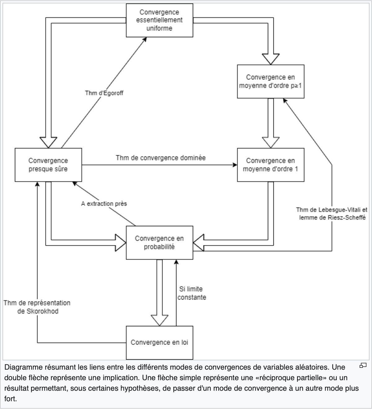
See this diagram (in french):
See: