Revision

Back to Finance - General

Definition

Bootstrapping is a method used to compute zero rate curves from incremental (in maturity) non zero rate instruments.

Bootstrapping aims at finding incrementally the zero rates using:

• The precedent zero rates,
• A non zero rate instrument.

The different instruments used to bootstrap a curve are:

• Spot value of the rate,
• Forward Rate Agreement,
• Interest Rate Swap (IRS),
• Bonds.

Single-Curve Framework vs Multi-Curve Framework

In the pre-crisis era, the standard market practice was to construct a single interest rate yield curve (single curve framework). This single interest rate yield curve was constructed using liquid vanilla interest Libor rate instruments based on different tenors (it could mix 1M Libor instruments with 6M Libor instruments, …).
This was possible as every of the Libor rates were risk free.

However the crisis showed that these Libor rates were not risk free.
As shown in the second graph, the spread between a 6M ZC rate on Euribor 3M and Euribor 6M was greater than 0 (same for 12M ZC rate on Euribor 6M vs Euribor 12M).

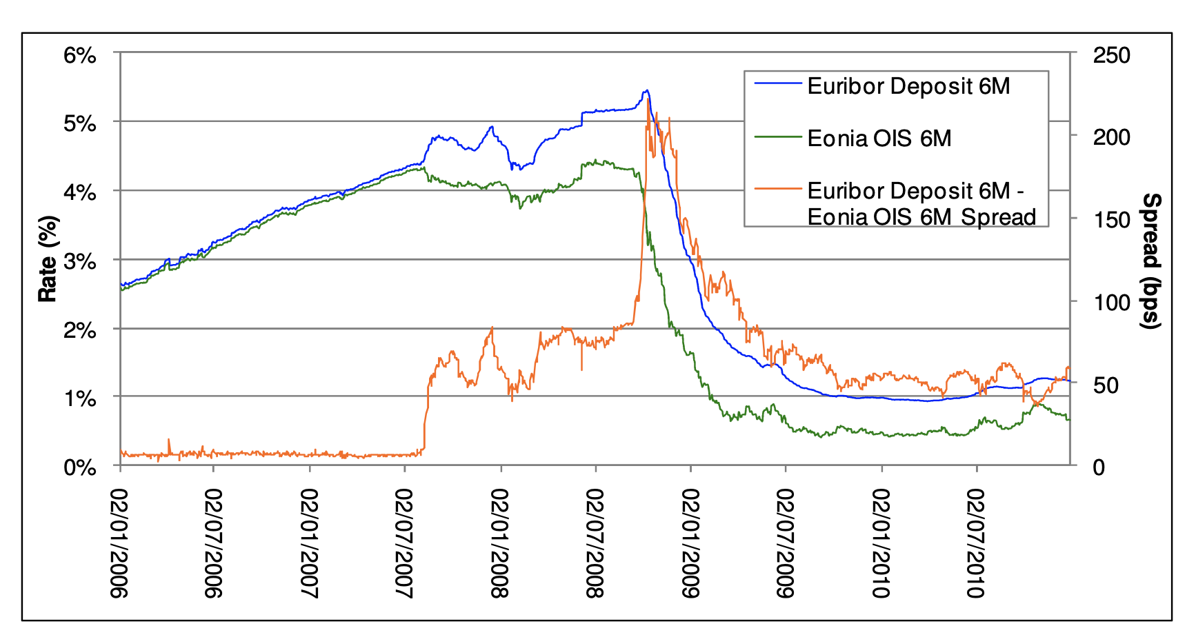
After the crisis the spread between EURIBOR and OIS curves started to increase, reflecting the risk premium in the EURIBOR rate.

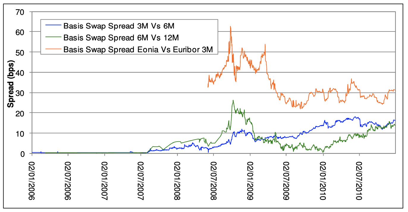
Also, after the crisis the temporal basis swap started to increase showing the greater credit risk associated with greater maturity.

This led to the creation of the multi curve framework where each rate (ESTR, Euribor 1M, Euribor 3M, Euribor 6M, Euribor 12M) induces its own yield curves and its own forward curves (forward curves that can be deducted from the spot yield curve).

Bootstraping Methodology

Bootstraping Methodology is the same in Single-Curve Framework and Multi-Curve Framework exept that in Multi-Curve Framework the discounted rate used is not the same as the rate of the instrument. This methodology is pretty straighforward.

For each point in time (maturity):

1. Retrieve market price of a non zero rate instrument with this maturity,
2. Retrieve past zero rates,
3. Use past zero coupon rates and market price of the instrument to deduce the zero coupon rate for this maturity.

Single-Curve Framework: Bootstrapping of OIS (Overnight Index Swap) Curve

Interest rate instrument are generally discounted using the OIS curve. Hence to bootstrap the OIS curve, the zero rate will appear in the discount factor as well as in the coupon definition.

Let \(DF(t,T) = e^{-r_{(t,T)}*(T-1)}\)

The pricing of the fixed/floating swap is:

Where:

• \(N\) is the swap nominal,
• \(C_{fixed}\) is the fixed coupon (the quoted or observable value),
• \(C_i\) is the OIS coupon (rate) between \(\left(T_{i-1}, T_i\right)\),
• \(\Delta\left(T_{i-1}, T_i\right)\) is the year fraction between \(T_{i-1}\) and \(T_i\).

Note that:

With:

• \(f_{T_j}\)t the (unobserved) fixing of the Overnight rate (for Overnight rate the fixings are daily when the coupon frequency is not).

The optimisation solves the following equation:

By finding the \(C_i\).
Finding the \(C_i\) is equivalent to finding the \(r_{(T_{i-1},T_i)}\) (equivalent to finding the product of the \(f_j\)).
The \(DF(t, T_i)\) are initially unknown and are totally linked to the \(r_{(T_{i-1},T_i)}\).

Generally we can assume a structure for the rates between two time periods \(T_i\) and \(T_{i+1}\) (for example constant rates on the period or using interpolation methods).

Using the Bootstrapping idea:

• We first use the quote of an OIS of maturity \(T_1\) and we look for \(C_1\) (and hence \(DF(t, T_1)\)) as it does not depend on the other \(C_i\),
• Then by recurrence, assuming \(C_i\) known, we use the quote of an OIS of maturity \(T_{i+1}\) and we look for \(C_{i+1}\) (and hence \(DF(t, T_{i+1})\)),
• We stop when we reach the last OIS instrument of maturity \(T_n\).

Using the obtained \(DF\) we can deduct the OIS zero rate curve.

Multi-Curve Framework: Bootstrapping of IBOR Curves

In the multi-curve framework, the discounting curve comes from a different (already bootstraped) curve than the one currently bootstraped.

Using FRA

The pricing of a FRA is:

To use the Bootstrapping method, the \(FRA(t, T_1, T_2)\) should be quoted (observable).
Then iteratively we find the \(r_{t,T_i}\) assuming \(r_{t,T_{i-1}}\) is known (\(r{t,T_1}\) is the observable value of the rate). The \(DF\) comes from another curve (OIS curve) and are already calculated.

Using Vanilla Interest Rate Swap (IRS)

To bootstrap IBOR products using vanilla swaps, the idea is the same than for the Overnight rate but here the discount factor comes for another already know zero rate discounting curve (the OIS discounting curve).

Where:

• \(N\) is the swap nominal,
• \(C_{fixed}\) is the fixed coupon (the quoted or observable value),
• \(C_i\) is the floating (IBOR) coupon (rate) between \(\left(T_{i-1}, T_i\right)\),
• \(\Delta\left(T_{i-1}, T_i\right)\) is the year fraction between \(T_{i-1}\) and \(T_i\).

Note that:

With:

• \(f_{T_j}\)t the (unobserved) fixing of the rate (the fixings of the rate may be different from the coupon frequency).

The optimisation solves the following equation:

By finding the \(C_i\).
Finding the \(C_i\) is equivalent to finding the \(r_{(T_{i-1},T_i)}\) (equivalent to finding the product of the \(f_j\)).
The \(DF\) comes from another curve (OIS curve) and are already calculated.

Real World example with Euribor 6M Bootstrap

Assume the OIS (ESTR) zero curve is already known.
Let see how the bootstrapping of the Euribor 6M is done.

For maturity from 1 week to 6 months

Use the observable rates of liquid Euribor products such as EUR001W for 1 week, EUR003M for 3 months or EUR006M for 6 months.

For maturity from 7 months to 18 months

Use the observable FRA quotations (from EUFR0AG for FRA(1M, 7M) to EUFR011F for FRA(12M, 18M)) and use the bootstrapping methodology for FRA products.

For maturity from 2 years to 50 years

Use the observable quotation of IRS (from EUSA2 for 2 years IRS to EUSA50 for 50 years IRS) and use the bootstrapping methodology for Vanilla IRS.

Bootstrapping of Multi Devise Curves

XCCY Basis Swaps

When pricing multi devise products, we could simply discount each leg given the discounting curve of its currency and then transform the foreign currency leg present value in the local currency using the spot FX rate.

However a basis spread exist when discounting the foreign leg. This spread expresses the difference in liquidity (balance) and credit risk of the two currency.

From Frontier advisors document on XCCY basis Swap: “In principle, the basis should be zero if access to funding in the two currencies is equal, unless there is a higher degree of credit risk imbedded in one index relative to another. However, companies do not have the same access to funding markets in multiple currencies. Financial and credit conditions differ across markets. The cross-currency basis spread therefore represents equilibrium in the supply of and demand for funding across different currencies, adjusted for the creditworthiness of the banks that generate the underlying floating index.”

A cross-currency basis swap hence represent a floating-for-floating exchange of interest rate payments in two different currencies. Unlike other basis swaps, they also exchange notional principals.
The XCCY Basis Swaps spread is an added value payed by the foreign leg (this spread can be negative).

Bootstrapping

To bootstrap a XCCY basis swap we should know:

• The local IBOR zero rate curve used in the XCCY basis swap (generally IBOR 3M),
• The foreign IBOR zero rate curve used in the XCCY basis swap (generally IBOR 3M),
• The local OIS curve.

The pricing of a XCCY basis swap is:

Where:

• \(FX(t)\) is the spot FX rate,
• \(N\) is the swap nominal,
• \(C_i^{local}\) is the floating (IBOR) coupon (rate) of the local currency between \(\left(T_{i-1}, T_i\right)\),
• \(C_i^{foreign}\) is the floating (IBOR) coupon (rate) of the foreign currency between \(\left(T_{i-1}, T_i\right)\),
• \(s\) is the quoted (observable) basis spread
• \(\Delta\left(T_{i-1}, T_i\right)\) is the year fraction between \(T_{i-1}\) and \(T_i\).

The optimisation solves the following equation:

By finding the \(DF_{CSA}\).
In the XCCY basis swap, the \(C_i^{local}\) and \(C_i^{foreign}\) are already known.

Reference

See:

• The Multi-Curve Framework: A Practitioner’s Guide,
• Frontier advisors document on XCCY basis Swap,
• Interest-Rate Modeling with Multiple Yield Curves by Pallavicini and Tarenghi,
• Credit Suisse Research: Cross-Currency Basis Swap.