Revision

Back to Inferential statistics

Definition

ANOVA for Analysis of Variance is a method to the impact of one ore more quantitive variables on a qualitative observed variable.

ANOVA analyzes the variances intra-class vs the variance inter-classes. To summarize, if the variances intra-class are low but the variance inter-classes is high then it the classes have an impact otherwise, if the variances intra-class and the variance inter-classes are similar then it is probable that the classes do not have an impact.

ANOVA uses the Fisher test to test the ratio of the variances.

Formula

The ANOVA model can have a fixed (deterministic) effect for each class of a random effect.

The formula for a fixed effect is the following:

\[y_{i,j}=A_i+\varepsilon_j\]

With:

i: the group number
j: the observation number in the group

The formula for a random effect is the following:

\[y_{i,j}=\alpha_i+\varepsilon_j\]

Where:

\(\alpha_i = mu_i + \varepsilon_i\) is a random effect and \(\varepsilon_i \sim \mathcal{N}(0, \sigma^2_i)\)

Assumptions

Samples are from a same population,
Observations are independent,
Distributions of the samples (or equivalently of the residuals) are normal,
Distributions are homoscedastics; to test homoscedasticity see Bartlett’s test,
\(\varepsilon_i \sim \mathcal{N}(0, \sigma^2)\).

Hypotheses to test

The tests used are the same for fixed and random effect but the formulation of the hypotheses are different.

Fixed effect

The hypotheses H0 says that the offsets \(A_i\) of every groups are equivalent.

H1 says that at least one group’s offset is different.

Fixed effect

The hypotheses H0 says that the variance of the random effect distribution is null (ie the expected values of the effects of each group are the same). H1 says that at this variance is not null.

Variance decomposition

An important law used in ANOVA is the law of total variance. Law of total variance says that \(Var(Y)=\mathbb{E}[Var(Y|X)] + Var(\mathbb{E}[Y|X])\).

The proof is based on the law of total expectation \(\mathbb{E}[Y]=\mathbb{E}[\mathbb{E}[Y \vert X]]\) and the definition of variance (see the proof on Wikipedia).

In ANOVA the law of total variance is used to express total variance from inter-classes variance and intra-classes variance. It is applied on sum of squares (that is not exactly the variance as not divided by the sample sizes):

\[SS_{Total}=SS_{Factors}+SS_{Residual}\]

Where:

\(SS_{Total}=\sum_{i=1}^{n_{pop}}\sum_{j=1}^{m_{obs}(i)}\left(y_{i, j}-\bar{y}\right)^2\),
\(SS_{Factors}=\sum_{i=1}^{n_{pop}}\left(\bar{y_i}-\bar{y}\right)^2\),
\(SS_{Residual}=\sum_{i=1}^{n_{pop}}\left(\sum_{j=1}^{m_{obs}(i)}\left(y_{i, j}-\bar{y_i}\right)^2\right)\).
\(n_{pop}\) is the number of groups,
\(m_{obs}(i)\) is the number of observation in the group i,
\(y_{i, j}\) is the j-th observation in group i,
\(\bar{y}\) is the global mean: \(\bar{y}=\frac{1}{n}\sum_{i=1}{n_{pop}}\sum_{j=1}{n_{obs}(i)}y_{i,j}\),
\(\bar{y_i}\) is the mean of group i: \(\bar{y_i}=\frac{1}{n_{obs}(i)}\sum_{j=1}{n_{obs}(i)}y_{i,j}\).

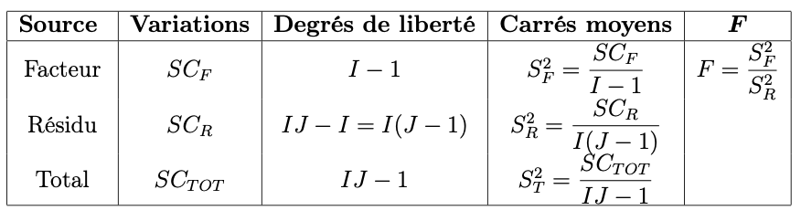
We also defined the mean squares:

\(S^2_{Total}=\frac{SS_{Total}}{n-1}\),
\(S^2_{Factors}=\frac{SS_{Factors}}{n_{pop}-1}\),
\(S^2_{Residual}=\frac{SS_{Residual}}{n-n_{pop}}\).

Distributions of the variances

Under the normality hypotheses and the hypotheses of equivalence of variances we have:

\(\frac{SS_{Total}}{\sigma} \sim \chi^2_{n-1}(X)\),
\(\frac{SS_{Factors}}{\sigma} \sim \chi^2_{n_{pop}}(X)\),
\(\frac{SS_{Residual}}{\sigma} \sim \chi^2_{n-n_{pop}}(X)\).

Fisher statistic

Using the distributions of \(SS_{Factors}\) and \(SS_{Residual}\) and the fact that the variances are equivalent, we obtain the Fisher statistic:

\[F = \frac{SS_{Factors}/(n_{pop}-1)}{SS_{Residual}/(n-n_{pop})}\]

And \(F \sim \mathcal{F}(n_{pop}-1, n-n_{pop})\).

We can then use the inverse cdf of the Fisher distribution on this value to obtain the test p-value.

Summary (in french)

Multi factors Analysis

If factors are independent, it is possible to make a multi factor analysis based on the same formula:

\[SS_{Total}=\sum_{f=1}^{n_{factors}}SS_{Factors_f}+SS_{Residual}\]

If the factors are not independent, the analysis of interactions among factors may be complex. For 2 factors, the formula would be:

\[SS_{Total}=SS_{Factors_1}+SS_{Factors_2}+SS_{Interaction}+SS_{Residual}\]

Where:

\[SS_{Interaction}=n\sum_{i_1=1}^{n_{pop_1}}\sum_{i_2=1}^{n_{pop_2}}\left(\bar{y_{(i_1, i_2)}}-\bar{y_{i_1}}-\bar{y_{i_2}}+\bar{y}\right)^2\]

Proof of \(SS_{Total}=SS_{Factors}+SS_{Residual}\)

Remark that \(y_{i,j}-\bar{y}=y_{i,j}-\bar{y_i}+\bar{y_i}-\bar{y}\) and that:

\[\begin{eqnarray} \left[y_{i,j}-\bar{y_i}+\bar{y_i}-\bar{y}\right]^2 && = \left[\left(y_{i,j}-\bar{y_i}\right)+\left(\bar{y_i}-\bar{y}\right)\right]^2 \\ && = \left(y_{i,j}-\bar{y_i}\right)^2+2\left(y_{i,j}-\bar{y_i}\right)\left(\bar{y_i}-\bar{y}\right)+\left(\bar{y_i}-\bar{y}\right)^2 \end{eqnarray}\]

Summing over all \(y_{i,j}\) we obtain: \(\begin{eqnarray} \sum_{i=1}^{n_{pop}}\sum_{j=1}^{m_{obs}(i)}\left[y_{i,j}-\bar{y_i}+\bar{y_i}-\bar{y}\right]^2 && = \sum_{i=1}^{n_{pop}}\sum_{j=1}^{m_{obs}(i)}\left[\left(y_{i,j}-\bar{y_i}\right)+\left(\bar{y_i}-\bar{y}\right)\right]^2 \\ && = \sum_{i=1}^{n_{pop}}\sum_{j=1}^{m_{obs}(i)}\left(y_{i,j}-\bar{y_i}\right)^2+2\sum_{i=1}^{n_{pop}}\sum_{j=1}^{m_{obs}(i)}\left(y_{i,j}-\bar{y_i}\right)\left(\bar{y_i}-\bar{y}\right)+\sum_{i=1}^{n_{pop}}\sum_{j=1}^{m_{obs}(i)}\left(\bar{y_i}-\bar{y}\right)^2 \\ && = \sum_{i=1}^{n_{pop}}\sum_{j=1}^{m_{obs}(i)}\left(y_{i,j}-\bar{y_i}\right)^2+\sum_{i=1}^{n_{pop}}\sum_{j=1}^{m_{obs}(i)}\left(\bar{y_i}-\bar{y}\right)^2 \end{eqnarray}\)

As \(2\sum_{i=1}^{n_{pop}}\sum_{j=1}^{m_{obs}(i)}\left(y_{i,j}-\bar{y_i}\right)\left(\bar{y_i}-\bar{y}\right) = 0\) as :

\[2\sum_{i=1}^{n_{pop}}\sum_{j=1}^{m_{obs}(i)}\left(y_{i,j}-\bar{y_i}\right)\left(\bar{y_i}-\bar{y}\right) = 2\sum_{i=1}^{n_{pop}}\left(\bar{y_i}-\bar{y}\right)\left[\sum_{j=1}^{m_{obs}(i)}\left(y_{i,j}-\bar{y_i}\right)\right]\]

And this is 0 as all \(\left[\sum_{j=1}^{m_{obs}(i)}\left(y_{i,j}-\bar{y_i}\right)\right]=0\) by definition of \(\bar{y_i}\).

References

See: