A/B testing is a methodology to test if two solutions A and B are equivalent when their outputs are non deterministic. A/B testing is widely used in online marketing to test if a design A is equivalent (or better or worse) than a design B for a given metric.
From a mathematical point of view A/B testing is just a practical application of statistical tests.
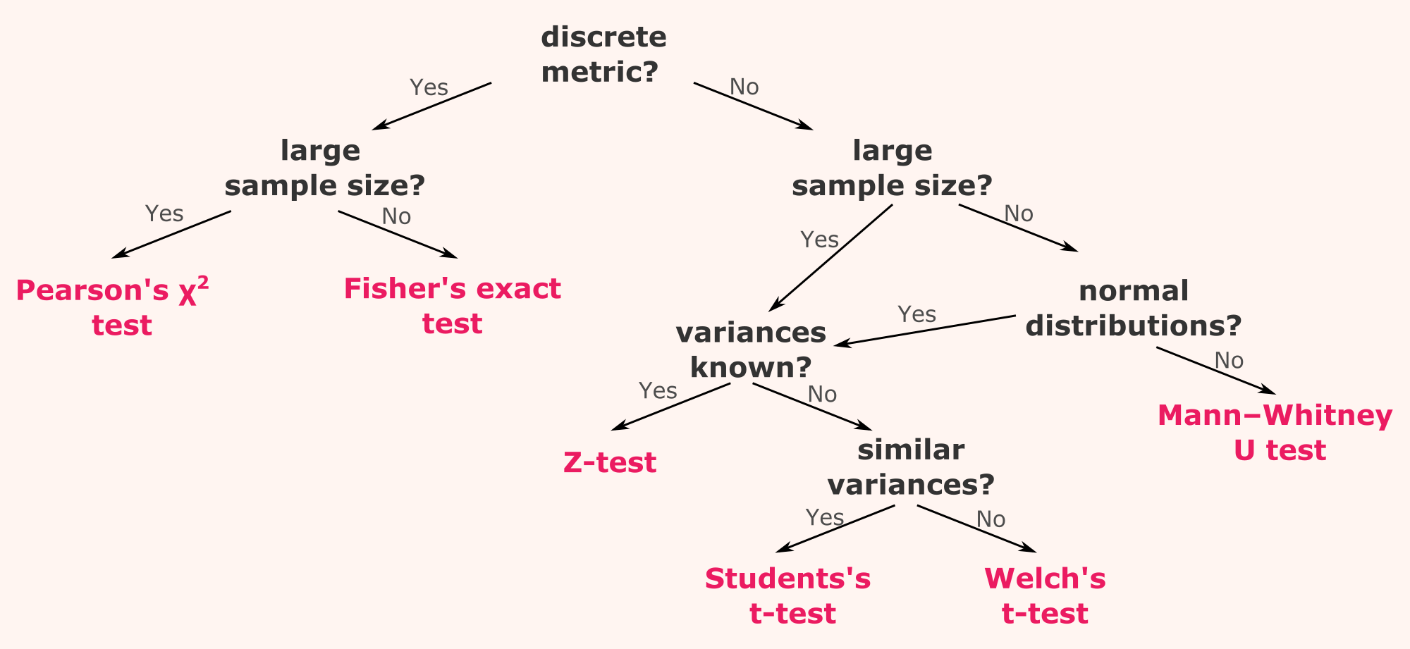
This image comes from a Toward Data Science blog post by Francesco Casalegno.
Different things may be tested in a two samples statistical test. We can check if A and B are equivalent or i A is better than B or if A is worse than B. The data type will decide which test to use (as you can see in the A/B Testing decision tree).
In online marketing, discret metrics may be:
These data are 0/1 data and they can be visualized in a cross tab.
This test is not used a lot because it is computationally inefficient with large sample sizes.
The Fisher exact test will compute all the possible permutations keeping the totals unchanged (total of users for A and for B and total of users who clicked or did not click).
Once all the permutations are available you can recompute, for each permutation, your metric for A and B (let’s say conversion rate). Your p-value is more or less the rank of your output (your output would be the difference of conversion rate between solution A and solution B) vs all the possible outputs. If you test if A is better than B then the permutation with higher \(CR_A-CR_B\) would represent the possible outcomes that are more extreme than the one we get.
This test is the one commonly used for categorical data. The idea is to compare the observed proportion to the expected proportion.
\[\chi^2=\sum_i\sum_j\frac{\left(O_{ij}-E_{ij}\right)^2}{E_{ij}}\]Where:
\(E_{ij}\) does correspond to the expected proportion under the assumption that A is equivalent to B. It is the case as its computation assumes that the correlation between the outcomes and the populations are null.
The degree of freedom of the Chi-2 distribution depends on the number of outcomes and the number of population. Its degree of freedom is \((nb_{populations}-1)(nb_{outcomes}-1)\). It the classical A/B testing framework this degree of liberty is 1.
A Chi-2 distribution is a sum of normally distributed variables. In this case the random variables are the \(O_{ij}\). It is thus expected that these \(O_{ij}\) follow a gaussian distribution.
\(O_{ij}\) is sum of Bernoulli random variables so \(O_{ij}\) is a Binomial random variable. More important, the Central limit theorem establishes that the sum of independent and identically distributed random variables converge in distribution toward the gaussian distribution (generally \(n \geq 30\) for every \(O_{ij}\)) so, for n large enough, \(O_{ij}\) follows a normal distribution (for n large enough, a Binomial distribution converges toward a normal distribution).
In online marketing, continuous metrics may be:
The Z-test checks if the means of two populations are equivalent. As for the Chi-2 distribution, the observations must follow a gaussian distribution or their sample sizes must be greater than 30 to be able to use the CLT. The variances of the population are known (which is generally not the case).
If the conditions are fulfilled, for two populations X and Y, the Z-statistic is written as follow:
\[Z=\frac{\bar{X}-\bar{Y}}{\sqrt{\frac{\sigma_X^2}{n_X} + \frac{\sigma_Y^2}{n_Y}}} \sim \mathcal{N}(0,1)\]The Student’s t-test gets the same assumptions as the Z-test but the variances will be estimated. In this case these variances are expected to be similar, ie \(\sigma_X \approx \sigma_Y\) (if it is not the case we can use the Welch’s t-test).
For two populations X and Y, the Student’s t-statistic is written as follow:
\[T=\frac{\bar{X}-\bar{Y}}{S_P\sqrt{\frac{1}{n_X} + \frac{1}{n_Y}}} \sim t_{\nu}\]Where:
The use of t-test is justified as \(\bar{X}-\bar{Y} \sim \mathcal{N}\) and \(S_P\sqrt{1/n_X + 1/n_Y} \sim \chi^2\) (a sum of squared gaussian distributed variables).
The Welch’s t-test is almost equivalent to the Student’s t-test but the variances are not considered equivalent. Thus we will estimate \(S^2_X\) and \(S^2_Y\) separately.
For two populations X and Y, the Welch’s t-statistic is written as follow:
\[T=\frac{\bar{X}-\bar{Y}}{\sqrt{\frac{S^2_X}{n_X} + \frac{S^2_Y}{n_Y}}} \sim t_{\nu}\]Where:
The Kolmogorov-Smirnov test is a non parametric test (ie without hypotheses in the data distribution). It is based on the empirical cumulative distribution function. It can be used to test if a sample of data follows a given distribution or in A/B testing if the distribution of data of each population are equivalent.
First let’s define the empirical functions: \(F_{n}(x)={\frac {\text{number of (elements in the sample} \leq x)}{n}}=\frac {1}{n}\sum_{i=1}^{n}1_{[-\infty ,x]}(X_{i})\)
Where:
Then the statistic in the Kolmogorov-Smirnov two samples test is computed as follow:
\[D_{n_X,n_Y}=\underset{x}{sup}|F_{1,n_X}(x)-F_{2,n_Y}(x)|\]Where:
The null hypotheses is rejected if:
\[D_{n_X,n_Y} \gt c(\alpha) \sqrt{\frac{n_X+n_Y}{n_X \cdot n_Y}}\]Where:
Mann–Whitney U test (or Wilcoxon-Mann-Whitney test) can be used for discrete or continuous data. It is a non parametric test.
For two populations X and Y, the Mann–Whitney U statistic is written as follow:
\[U=\sum_{i=1}^{n_X}\sum_{j=1}^{n_Y}D(X_i, Y_j)\]Where:
The hypotheses H0 is that the distributions of the populations X and Y are equivalent can be reformulate as follow: “the probability for an observation \(X_i\) of X to be greater than an observation \(Y_j\) of Y is equal to the probability for an observation \(Y_j\) of Y to be greater than an observation \(X_i\) of X”.
See: